The Laplace Operator
The Laplacian and its various forms in different coordinates.
- The Laplacian in polar coordinate
- The Laplacian in cylindrical coordinate
- The Laplacian in spherical coordinate
Let \(u\) be the function of \(x, y\) and its Laplacian is defined as the divergence of the gradient of \(u\) (w.r.t \(x, y\)), i.e., \(\nabla \cdot \nabla u\) and the Laplacian in Cartesian coordinate is given as
\[\begin{equation} \tag{laplacian}\label{eq:laplacian} \nabla \cdot \nabla u = \frac{\partial^2 u}{\partial x^2} + \frac{\partial^2 u}{\partial y^2}. \end{equation}\]Now we generalize the Laplacian into three different coordinates most commonly used in mathematical physics equations, namely, the polar coordinate, cylindrical coordinate, and spherical coordinate. The three coordinate systems characterize the Euclidean space from different perspective, and each of them has its unique convenience under different situations.
The Laplacian in polar coordinate
We have the transformation between the Cartesian coordinate and polar coordinate
\[\begin{equation} \tag{polar}\label{eq:polar} \begin{aligned} x &= r \cos \theta\\ y &= r \sin \theta. \end{aligned} \end{equation}\]To establish the Laplacian in the polar coordinate, we need to represent the Laplace operator \(\nabla \cdot \nabla\) in Eq. \eqref{eq:laplacian} with the variables \(r, \theta\). This is possible if we can represent \({\partial^2 u}/{\partial x^2}\) and \({\partial^2 u}/{\partial y^2}\) in terms of \({\partial^2 u}/{\partial r^2}\), \({\partial^2 u}/{\partial \theta^2}\), \({\partial u}/{\partial r}\), and \({\partial u}/{\partial \theta}\). To compute the second order partial derivative \({\partial^2 u}/{\partial x^2}\) and \({\partial^2 u}/{\partial y^2}\), we need to represent the first order partial derivative \({\partial u}/{\partial x}\) and \({\partial u}/{\partial y}\) with \({\partial u}/{\partial r}\) and \({\partial u}/{\partial \theta}\).
To this end, we treat \((x, y)\) as the independent variables and \((r, \theta)\) the intermediate variables, that is,
\[u \leftarrow (r, \theta) \leftarrow (x, y).\]According to the chain rule, we have
\[\begin{align} \frac{\partial u}{\partial x} &= \frac{\partial u}{\partial r} \frac{\partial r}{\partial x} + \frac{\partial u}{\partial \theta} \frac{\partial \theta}{\partial x}\\ \frac{\partial u}{\partial y} &= \frac{\partial u}{\partial r} \frac{\partial r}{\partial y} + \frac{\partial u}{\partial \theta} \frac{\partial \theta}{\partial y}. \end{align}\]This is a linear system of \({\partial u}/{\partial r}\) and \({\partial u}/{\partial \theta}\), whose coefficients form the transpose of Jacobian matrix \(\mathbf{J}_{r\theta/xy}\), defined as,
\[\mathbf{J}_{r\theta/xy} = \left[\begin{array}{cc} \frac{\partial r}{\partial x} & \frac{\partial r}{\partial y}\\ \frac{\partial \theta}{\partial x} & \frac{\partial \theta}{\partial y} \end{array}\right]\]Hence, we should find a way to calculate \({\partial r}/{\partial x}\) and \({\partial \theta}/{\partial x}\) as well as \({\partial r}/{\partial y}\) and \({\partial \theta}/{\partial y}\) first.
First, we find \({\partial r}/{\partial x}\), \({\partial \theta}/{\partial x}\), \({\partial r}/{\partial y}\), \({\partial \theta}/{\partial y}\) by differentiating \(x\) (resp. \(y\)) on both sides of Eq. \eqref{eq:polar} to yield
\[\begin{alignat}{4} % 1 &= \frac{\partial x}{ \partial x}\ && = \frac{\partial (r \cos \theta)}{\partial x}\ &&&= \frac{\partial r}{\partial x}\cos \theta - \frac{\partial \theta}{\partial x}r \sin \theta \\ % 0 &= \frac{\partial y}{ \partial x}\ && = \frac{\partial (r \sin \theta)}{\partial x}\ &&&= \frac{\partial r}{\partial x}\sin \theta + \frac{\partial \theta}{\partial x}r \cos \theta \\ \end{alignat}\]and
\[\begin{alignat}{4} % 0 &= \frac{\partial x}{ \partial y}\ && = \frac{\partial (r \cos \theta)}{\partial y}\ &&&= \frac{\partial r}{\partial y}\cos \theta - \frac{\partial \theta}{\partial y}r \sin \theta \\ % 1 &= \frac{\partial y}{ \partial y}\ && = \frac{\partial (r \sin \theta)}{\partial y}\ &&&= \frac{\partial r}{\partial y}\sin \theta + \frac{\partial \theta}{\partial y}r \cos \theta \end{alignat}\]from which we can establish two linear equations
\[\left[\begin{array}{cc} \cos \theta & - r \sin \theta \\ \sin \theta & r\cos \theta \\ \end{array}\right] \left[\begin{array}{c} \frac{\partial r}{\partial x} \\ \frac{\partial \theta}{\partial x} \end{array}\right] = \left[\begin{array}{c} 1 \\ 0 \end{array}\right]\]and
\[\left[\begin{array}{cc} \sin \theta & r \cos \theta \\ \cos \theta & -r\sin \theta \\ \end{array}\right] \left[\begin{array}{c} \frac{\partial r}{\partial y} \\ \frac{\partial \theta}{\partial y} \end{array}\right] = \left[\begin{array}{c} 1 \\ 0 \end{array}\right].\]By solving the two equations we can obtain
\[\left[\begin{array}{c} \frac{\partial r}{\partial x} \\ \frac{\partial \theta}{\partial x} \end{array}\right] = \left[\begin{array}{c} \cos \theta \\ -\frac{1}{r}\sin \theta \end{array}\right],\ \left[\begin{array}{c} \frac{\partial r}{\partial y} \\ \frac{\partial \theta}{\partial y} \end{array}\right] = \left[\begin{array}{c} \sin \theta \\ \frac{1}{r} \cos \theta \end{array}\right]\]or more compactly as the Jacobian matrix
\[\begin{equation} \tag{jacobian}\label{eq:jacobian} \mathbf{J}_{r\theta/xy} = \left[\begin{array}{cc} \frac{\partial r}{\partial x} & \frac{\partial r}{\partial y}\\ \frac{\partial \theta}{\partial x} & \frac{\partial \theta}{\partial y} \end{array}\right] = \left[\begin{array}{cc} \cos \theta & \sin \theta\\ -\frac{1}{r}\sin \theta & \frac{1}{r} \cos \theta\end{array}\right]. \end{equation}\]There is a more convenient method to calculate \(\mathbf{J}_{r\theta/xy}\) by first computing the Jacobian matrix of \(\mathbf{J}_{xy/r\theta}\)
\[\mathbf{J}_{xy/r\theta} = \left[\begin{array}{cc} \frac{\partial x}{\partial r} & \frac{\partial x}{\partial \theta}\\ \frac{\partial y}{\partial r} & \frac{\partial y}{\partial\theta} \end{array}\right] = \left[\begin{array}{cc} \cos \theta & -r \sin \theta\\ \sin \theta & r \cos \theta\end{array}\right]\]and then applying the inverse function theorem to yield \(\mathbf{J}_{r\theta/xy} = \mathbf{J}_{xy/r\theta}^{-1}\).
Next, we use the chain rule to express \(\frac{\partial u}{\partial x}\) with \(\frac{\partial u}{\partial r}\) and \(\frac{\partial u}{\partial \theta}\),
\[\frac{\partial u}{\partial x} = \frac{\partial u}{\partial r} \frac{\partial r}{\partial x} + \frac{\partial u}{\partial \theta} \frac{\partial \theta}{\partial x} = \frac{\partial u}{\partial r} \cos \theta - \frac{\partial u}{\partial \theta} \frac{1}{r} \sin \theta\]and differentiating w.r.t \(x\) once more to produce
\[\frac{\partial^2 u}{\partial x^2} = \frac{\partial^2 u}{\partial r^2} \cos^2 \theta - \frac{\partial^2 u}{\partial r \partial \theta} \frac{2}{r} \sin \theta \cos \theta + \frac{\partial^2 u}{\partial \theta^2} \frac{1}{r^2} \sin^2 \theta + \frac{\partial u}{\partial r} \frac{1}{r} \sin^2 \theta + \frac{\partial u}{\partial \theta} \frac{2}{r^2} \cos \theta \sin \theta.\]Similarly, we can compute
\[\frac{\partial^2 u}{\partial y^2} = \frac{\partial^2 u}{\partial r^2} \sin^2 \theta + \frac{\partial^2 u}{\partial r \partial \theta} \frac{2}{r} \sin \theta \cos \theta + \frac{\partial^2 u}{\partial \theta^2} \frac{1}{r^2} \cos^2 \theta + \frac{\partial u}{\partial r} \frac{1}{r} \cos^2 \theta - \frac{\partial u}{\partial \theta} \frac{2}{r^2} \cos \theta \sin \theta.\]By combining the two equations, we get
\[\begin{equation} \tag{polar-lap}\label{eq:polar-lap} \begin{aligned} \nabla \cdot \nabla w &= \frac{\partial^2 u}{\partial x^2} + \frac{\partial^2 u}{\partial y^2} = \frac{\partial^2 u}{\partial r^2} + \frac{1}{r^2}\frac{\partial^2 u}{\partial \theta^2} + \frac{1}{r}\frac{\partial u}{\partial r}\\ \nabla \cdot \nabla &= \frac{\partial^2 }{\partial r^2} + \frac{1}{r^2}\frac{\partial^2 }{\partial \theta^2} + \frac{1}{r}\frac{\partial}{\partial r} \end{aligned} \end{equation}\]The Laplacian in cylindrical coordinate
In the cylindrical coordinate, we have
\[\begin{aligned} x &= \rho \cos \theta\\ y &= \rho \sin \theta\\ z &= z \end{aligned}\]where we use \(\rho, \theta\) to identify the polar coordinate corresponding to the \(xy\)-plane by following the mathematics convention (it is \(\rho, \phi\) by the physcis convention). It is straightforward to generalize the Laplacian to the cylindrical coordinate since \(z\) is independent from the \(xy\)-plane whose polar coordinate Laplacian is exactly what we have established.
\[\begin{aligned} \nabla \cdot \nabla u &= \frac{\partial^2 u}{\partial x^2} + \frac{\partial^2 u}{\partial y^2} + \frac{\partial^2 u}{\partial z^2} = \frac{\partial^2 u}{\partial \rho^2} + \frac{1}{\rho^2}\frac{\partial^2 u}{\partial \theta^2} + \frac{1}{\rho}\frac{\partial u}{\partial \rho} + \frac{\partial^2 u}{\partial z^2}\\ \nabla \cdot \nabla &= \frac{\partial^2}{\partial \rho^2} + \frac{1}{\rho^2}\frac{\partial^2}{\partial \theta^2} + \frac{1}{\rho}\frac{\partial}{\partial \rho} + \frac{\partial^2}{\partial z^2}\\ \end{aligned}\]The Laplacian in spherical coordinate
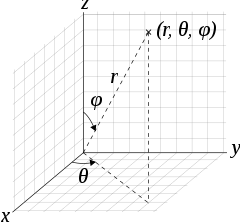
In the spherical coordinate, we have
\[\begin{aligned} x &= r \sin \phi \cos \theta\\ y &= r \sin \phi \sin \theta\\ z &= r \cos \phi \end{aligned}\]which can be viewed as two orthogonal planes \(xy\)-plane and \(\rho z\)-plane with \(\rho = r \sin \phi\). Thus, we can apply what we have established in Eq. \eqref{eq:polar-lap} to the two planes, respectively, to yield
\[\begin{aligned} \frac{\partial^2 u}{\partial x^2} + \frac{\partial^2 u}{\partial y^2} &= \frac{\partial^2 u}{\partial \rho^2} + \frac{1}{\rho^2}\frac{\partial^2 u}{\partial \theta^2} + \frac{1}{\rho}\frac{\partial u}{\partial \rho} \\ \frac{\partial^2 u}{\partial z^2} + \frac{\partial^2 u}{\partial \rho^2} &= \frac{\partial^2 u}{\partial r^2} + \frac{1}{r^2}\frac{\partial^2 u}{\partial \phi^2} + \frac{1}{r}\frac{\partial u}{\partial r} \end{aligned}\]By adding both sides of the two equations and rearranging the terms, we have
\[\begin{equation} \tag{spherical-lap0}\label{eq:spherical-lap} \frac{\partial^2 u}{\partial x^2} + \frac{\partial^2 u}{\partial y^2} + \frac{\partial^2 u}{\partial z^2} = \frac{\partial^2 u}{\partial r^2} + \frac{1}{r^2}\frac{\partial^2 u}{\partial \phi^2} + \frac{1}{\rho^2}\frac{\partial^2 u}{\partial \theta^2} + \frac{1}{\rho}\frac{\partial u}{\partial \rho} + \frac{1}{r}\frac{\partial u}{\partial r} \end{equation}\]To obtain the Laplacian in spherical coordinate, we only need to eliminate \(\rho\) and \({\partial u}/{\partial \rho}\) from the right side. \(\rho = r \sin \phi\) whereas
\[\frac{\partial u}{\partial \rho} = \frac{\partial u}{\partial r} \frac{\partial r}{\partial \rho} + \frac{\partial u}{\partial \phi} \frac{\partial \phi}{\partial x} = \frac{\partial u}{\partial r} \sin \phi + \frac{\partial u}{\partial \phi} \frac{1}{r} \cos \phi\]the first equaltiy is established by applying the chain rule to \(w\) in the \(\rho z\)-plane and the second equality is obtained by observing the Jacobian matrix in Eq. \eqref{eq:jacobian} and treating \(\rho\) to \(y\) and \(\phi\) to \(\theta\).
Now replacing \(\rho\) and \({\partial u}/{\partial \rho}\) into Eq. \eqref{eq:spherical-lap}, we get
\[\begin{aligned} \nabla \cdot \nabla u &= \frac{\partial^2 u}{\partial r^2} + \frac{1}{r^2}\frac{\partial^2 u}{\partial \phi^2} + \frac{1}{r^2 \sin^2 \phi}\frac{\partial^2 u}{\partial \theta^2} + \frac{1}{r \sin \phi} \left(\frac{\partial u}{\partial r} \sin \phi + \frac{\partial u}{\partial \phi} \frac{1}{r} \cos \phi \right) + \frac{1}{r}\frac{\partial u}{\partial r}\\ &= \frac{\partial^2 u}{\partial r^2} + \frac{2}{r}\frac{\partial u}{\partial r} + \frac{1}{r^2}\frac{\partial^2 u}{\partial \phi^2} + \frac{1}{r^2} \cot \phi \frac{\partial u}{\partial \phi} + \frac{1}{r^2 \sin^2 \phi}\frac{\partial^2 u}{\partial \theta^2}\\ &= \frac{\partial^2 u}{\partial r^2} + \frac{2}{r}\frac{\partial u}{\partial r} + \frac{1}{r^2 \sin \phi}\frac{\partial }{\partial \phi}\left(\frac{\partial u}{\partial \phi} \sin \phi\right) + \frac{1}{r^2 \sin^2 \phi}\frac{\partial^2 u}{\partial \theta^2}\\ \nabla \cdot \nabla &= \frac{\partial^2}{\partial r^2} + \frac{2}{r}\frac{\partial}{\partial r} + \frac{1}{r^2}\frac{\partial^2 }{\partial \phi^2} + \frac{1}{r^2} \cot \phi \frac{\partial}{\partial \phi} + \frac{1}{r^2 \sin^2 \phi}\frac{\partial^2}{\partial \theta^2}\\ &= \frac{\partial^2 }{\partial r^2} + \frac{2}{r}\frac{\partial }{\partial r} + \frac{1}{r^2 \sin \phi}\frac{\partial }{\partial \phi}\left(\frac{\partial }{\partial \phi} \sin \phi\right) + \frac{1}{r^2 \sin^2 \phi}\frac{\partial^2 }{\partial \theta^2}\\ \end{aligned}\]