Daily Collection
Random topics from analysis, algebra, geometry, probability, etc.
Analysis & Probability
Limit superior and limit inferior
For a collection of set \(\{E_n\}\),
\[\limsup E_n = \bigcap_{k=1}^\infty \bigcup_{n=k}^\infty E_n,\] \[\liminf E_n = \bigcup_{k=1}^\infty \bigcap_{n=k}^\infty E_n.\]\(\limsup\) on set collection means union starting from infinity \(\bigcup_{n \geq N}^\infty\) and \(\liminf\) means intersection starting from infinity \(\bigcap_{n \geq N}^\infty\).
For a sequence of \(\{x_n\}\),
\[\limsup x_n = \inf_{k \geq 1} \sup_{n \geq k} x_n,\] \[\liminf x_n = \sup_{k \geq 1} \inf_{n \geq k} x_n.\]Cantor set
Let \(F_0\) be the interval \([0, 1]\). We remove the open interval \((\frac{1}{3}, \frac{2}{3})\) from \(F_0\) and denote the remaining closed set by \(F_1\). Then we remove the middle interval of length \(\left(\frac{1}{3}\right)^2\) from each of the two intervals of \(F_1\) and denote the remaining closed set by \(F_2\) and so forth as the Figure Cantor Set shown.
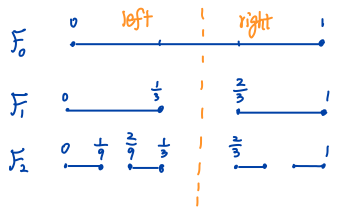
Figure Cantor Set
Note that we can scale \(F_0\) by \(\frac{1}{3}\) to get the left part of \(F_1\) and then shift the left part by \(\frac{2}{3}\) to get the right part, that is,
\[F_1 = \frac{1}{3} F_0 \bigcup \left(\frac{1}{3} F_0 + \frac{2}{3}\right).\]Similarly, if we scale \(\left[0, \frac{1}{3}\right]\) and \(\left[\frac{2}{3}, 1\right]\) by \(\frac{1}{3}\) we could map them to intervals \(\left[0, \frac{1}{9}\right]\) and \(\left[\frac{2}{9}, \frac{1}{3}\right]\), respectively. The two intervals are exactly the left part of \(F_2\) and we can shift them by \(\frac{2}{3}\) to get the right part of \(F_2\), that is,
\[F_2 = \frac{1}{3} F_1 \bigcup \left(\frac{1}{3} F_1 + \frac{2}{3}\right).\]Note that the left part of \(F_2\) is still ranging from \(0\) to \(\frac{1}{3}\) and if we scale it by \(\frac{1}{3}\) we map these intervals into \(\left[0, \frac{1}{9}\right]\) again. Also, the right part of \(F_2\) will be mapped into \(\left[\frac{2}{9}, \frac{1}{3}\right]\) by scaling \(\frac{1}{3}\). This implies,
\[F_n = \frac{1}{3} F_{n-1} \bigcup \left(\frac{1}{3} F_{n-1} + \frac{2}{3}\right),\]holds for \(n = 1, 2, \ldots\).
The Cantor set is defined as \(F = \bigcap_{n=0}^{\infty} F_n\). If we represent all numbers in \([0, 1]\) in the triadic system, that is, \(\frac{1}{3} a_1 + \frac{1}{3^2} a_2 + \ldots\) where \(a_n \in \{0, 1, 2 \}\). Each \(x \in [0, 1]\) can be represented by a sequence of \(a_1, a_2, \ldots\), and
\[\begin{aligned} 0 &= 0, 0, \ldots\\ 1 &= 2, 2, \ldots \end{aligned}\]For a \(x = a_1, a_2, \ldots\) we can interpret the operations \(g\) of the following
\[\begin{aligned} \frac{1}{3} &\longrightarrow 0, a_1, a_2, \ldots\\ \frac{1}{3}x + \frac{2}{3} &\longrightarrow 2, a_1, a_2, \ldots \end{aligned}\]as prepending 0 and 2 to the sequence \(a_n\), respectively.
Starting from sequences \(0, 0, \ldots\), \(2, 2, \ldots\) and transforming sequences using the above two operations we could generate all possible sequences consisting of 0 and 2. In other words,
\[F \stackrel{g}{\longrightarrow} \text{all possible sequences of 0, 2}.\]However, the set of such sequences has the power of the continuum, which can be observed by replacing 2 to 1 and the set corresponds to a binary representation of all numbers in \([0, 1]\). Hence, given any \(x \in [0, 1]\) its preimage in \(F\) is unique. This implies that \(F\) has cardinal number not less than the cardinal number of the continuum.
Convergence in probability and distribution
A sequence of random variables \(X_1, X_2, \ldots,\) converge in probability to a random variable \(X\), that is, \(X_n \stackrel{p}{\rightarrow} X\), if
\[\lim_{n \rightarrow \infty} \mathbb{P} (\vert X_n - X \vert \geq \epsilon) = 0 \quad \text{for all } \epsilon > 0.\]A sequence of random variables \(X_1, X_2, \ldots,\) converge in distribution to a random variable \(X\), that is, \(X_n \stackrel{d}{\rightarrow} X\), if
\[\lim_{n \rightarrow \infty} F_{X_n}(x) = F_X(x),\]for all \(x\) at which \(F_X(x)\) is continuous.
Example. Let \(X_1, X_2, \ldots,\) be a sequence of random variable such that
\[X_n \sim \mathrm{Binomial}(n, \frac{\lambda}{n}) \quad \text{for } n \in \mathbb{N}, n > \lambda > 0,\]then \(X_n\) converges in distribution to \(\mathrm{Poisson}(\lambda)\).
NTU bus arrival problem
Suppose Bus 179 arrives every 5 minutes, Bus 199 arrives every 20 minutes and you arrive bus station randomly, what is the probability of 199 arrives first?
Let \(x\) and \(y\) be the arrival time of 199 and 179 in a time interval \([0, 20]\), \(A\) be the event of 199 arriving first. By the assumption, the event of 179 arriving must happen within the first 5 minutes therefore \(A \Longleftrightarrow 0 < x < y < 5\) and
\[\mathbb{P}(A) = \int_0^5 \int_x^5 \frac{1}{5} dy \frac{1}{20} dx = \frac{1}{8}.\]Dice rolling problem
Let \(X\) be the number of steps taken to observe two consecutive 6 when rolling a fair dice, what is its distribution?
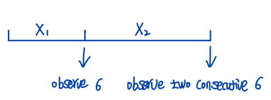
Figure Dice Rolling
Since we need to roll at least two times to observe two consecutive 6, \(X-1\) is a geometric distribution. Let \(X_1\) be the number of steps taken to see the first 6 and \(X_2\) be the number of steps taken to see two consecutive 6 after we have observed the first 6, and \(A\) be the event of observing 6 in the next step when 6 is observed in the present step. Then, \(X = X_1 + X_2\) and
\[\begin{aligned} \mathbb{E}[X] &= \mathbb{E}[X_1] + \mathbb{E}[X_2],\\ \mathbb{E}[X_1] &= 6,\\ \mathbb{E}[X_2] &= \mathbb{E}[X_2 \vert A = 1] \mathbb{P}(A = 1) + \mathbb{E}[X_2 \vert A = 0] \mathbb{P}(A = 0)\\ &= 1 \times \frac{5}{6} + (\mathbb{E}[X] + 1) \times \frac{1}{6}. \end{aligned}\]Solving the equation, we obtain \(\mathbb{E}[X] = 42\). Hence, \(Y = X-1\) is a geometric distribution with \(\mathbb{E}[Y] = 41\) or success probability \(p = 1/41\),
\[\mathbb{P}(X = k) = \mathbb{P}(Y = k - 1) = (1-p)^{k-2} p, \quad k = 2, 3, \ldots\]Coupon collector problem
When we have collected \(k\) distinct coupons, the probability of getting a new coupon is \(\frac{n-k}{n}\). Clearly, the number of steps \(X_k\) required to take to get the new one follows a geometric distribution with success probability \(\frac{n-k}{n}\) and \(\mathbb{E}X_k = \frac{n}{n - k}.\)
Hence, the expected total number of steps needed to collect all coupons is
\[\begin{aligned} \mathbb{E}\left[\sum_{k=0}^{n-1} X_k\right] &= \sum_{k=0}^{n-1}\mathbb{E}[X_k]\\ &= \sum_{k=0}^{n-1} \frac{n}{n-k} = \sum_{k=1}^{n} \frac{n}{k} \\ &= n\left(1 + \frac{1}{2} + \ldots + \frac{1}{n}\right) \approx n \log n. \end{aligned}\]Linear Algebra & Functional
Inner product in complex space
Suppose \(V\) is a vector space over the field \(\mathbb{C}\) and for \(v, {w} \in V\), the inner product is denoted by \(\langle v, w \rangle\). In analysis, the inner product is defined to be linear in the first argument and conjugate-linear in the second argument, that is,
\[\begin{aligned} \langle \lambda v, w \rangle &= \lambda \langle v, w \rangle\\ \langle v, \lambda w \rangle &= \bar{\lambda} \langle v, w \rangle. \end{aligned}\]However, in physics, in particular, quantum mechanics, the conjugate-linearity is defined for the first argument and the linearity is for the second argument,
\[\begin{aligned} \langle \lambda v, w \rangle &= \bar{\lambda} \langle v, w \rangle\\ \langle v, \lambda w \rangle &= \lambda \langle v, w \rangle. \end{aligned}\]The results given by the two definitions differ by a conjugate operation since inner product satisfies conjugate symmetry.
In both definitions, the properties we present for innner product in matrix-calculus hold by replacing transpose with conjugate transpose,
\[\begin{align} \langle AC, BD \rangle &= \langle B^* AC, D \rangle = \langle C, A^* BD \rangle \\ &= \langle A C D^*, B \rangle = \langle A, B D C^* \rangle. \end{align}\]Matrix norm
1-norm.
\[\begin{aligned} \| A \|_1 &= \sup_{\| x \|_1 = 1} \| A x \|_1 = \sup_{\| x \|_1 = 1} \| \sum_{j=1}^n x_j a_j \|_1 \\ &\leq \sup_{\| x \|_1 = 1} \sum_{j}\| x_j a_j \|_1 \leq \max_{1 \leq j \leq n} \| a_j \|_1 \end{aligned}\]where \(a_j\) is the \(j\)-column of \(A\) and the upper bound is attained when \(x\) put all energy in the column with the largest 1-norm.
Infinity norm.
\[\begin{aligned} \| A \|_\infty &= \sup_{\| x \|_\infty = 1} \| A x \|_\infty \\ &= \sup_{\| x \|_\infty = 1} \max_{1 \leq i \leq m} \vert a_i^* x \vert = \max_{1 \leq i \leq m} \sup_{\| x \|_\infty = 1} \vert a_i^* x \vert\\ &\leq \max_{1 \leq i \leq m} \sum_{j=1}^n |a_{ij}| = \max_{1 \leq i \leq m} \|a_i\|_1 \end{aligned}\]where \(a_i\) is the conjugate transpose of \(i\)-th row of \(A\) and the upper bound can be attained by setting \(x_j = e^{-i\theta_j}\) if \(\bar{a}_{ij} = r_j e^{i\theta_j}\) (actually \(x_j\) can be any value on the unit circle). We can also apply Hölder’s inequality in the second line to obtain the result, that is,
\[\sup_{\| x \|_\infty = 1} \vert a_i^* x \vert \leq \|a_i\|_1 \|x\|_\infty = \|a_i\|_1.\]Polynomial representation and FFT
A polynomial of degree \(n-1\) can be represented by \(n\) coefficient \(c_0, c_1, \ldots, c_{n-1}\) or its evaluated values at \(n\) distinct points.
\[\left[ \begin{array}{c} p(1)\\ p(x_1)\\ p(x_2)\\ \vdots\\ p(x_{n-1}) \end{array} \right] = \left[ \begin{array}{lllll} 1& 1& 1& \ldots& 1\\ 1& x_1& x_1^2&\ldots &x_1^{n-1}\\ 1& x_2& x_2^2&\ldots &x_2^{n-1}\\ \vdots&\vdots & \vdots& &\vdots\\ 1& x_{n-1}& x_{n-1}^2 & & x_{n-1}^{n-1} \end{array} \right] \left[ \begin{array}{c} c_0\\ c_1\\ c_2\\ \vdots\\ c_{n-1} \end{array} \right]\]Given two polynomials
\[\begin{aligned} p_1(x) &= a_0 + a_1 x + \ldots + a_{n-1} x^{n-1}, \\ p_2(x) &= b_0 + b_1 x + \ldots + b_{n-1} x^{n-1}. \end{aligned}\]The product of \(p_1\) and \(p_2\) is a polynomial of \(2n-2\) degree with \(2n-1\) coefficients \(c_0, c_1, \ldots, c_{2n-2}\) and \(c_k = \sum_{i=1}^k a_i b_{k-i}\). In other words, \(\mathbf{c} = \mathbf{a} \circledast \mathbf{b}\), the convolution of \(a\) and \(b\).
The convolution operation of two length \(n\) vectors is of complexity \(O(n^2)\). However, if we could represent \(p_1, p_2\) using their value representations, we only need to do elementwise multiplication of their values evaluated at \(2n-1\) distinct points and the result uniquely determines the polynomial \(p_1(x) \cdot p_2(x)\). In this case, we need to pad \(a\) and \(b\) with zeros to be length of \(2n-1\) like \([0, \ldots, 0, a_0, \ldots, a_{n-1}]^\top\) and \([0, \ldots, 0, b_0, \ldots, b_{n-1}]^\top\).
Hence, we could first transform the coefficient representation into the value representation by a linear map, and we can do elementwise product in the value representation to get \(p_1(x) \cdot p_2(x)\). Then we can get back to the coefficient representation by the inverse linear map. However, the linear map (inverse linear map) itself is very expensive \(O(n^2)\), so can we do better by carefully choosing the linear map?

Fig. Roots of Unity
The FFT (Fast Fourier Transform) choose the \(n\) distinct points to be \(\omega^0, \omega^1, \ldots, \omega^{n-1}\) where \(\omega = e^{2 \pi i/n}\), that is, the \(n\) unitary roots in the unit circle as shown in the Figure and the linear map is defined by matrix
\[\Omega = \frac{1}{\sqrt{n}}\left[\begin{array}{lllll} 1& 1& 1& \ldots& 1\\ 1& \omega^ {1 \cdot 1} & \omega^{1\cdot 2}&\ldots &\omega^{1\cdot (n-1)}\\ 1& \omega^{2 \cdot 1}& \omega^{2 \cdot 2}&\ldots &\omega^{2\cdot (n-1)}\\ \vdots&\vdots & \vdots& &\vdots\\ 1& \omega^{(n-1) \cdot 1}& \omega^{(n-1) \cdot 2} & & \omega^{(n-1)\cdot (n-1)} \end{array} \right]\]where we put a normalization factor \(\frac{1}{\sqrt{n}}\) such that \(\Omega\) is a unitary matrix, \(\Omega \Omega^* = I\).
Suppose \(n\) is the power of 2, the origin-symmetry pairs \((\omega^k, \omega^{k + n/2})\) in the unit circle
\[- \omega^k = e^{2\pi i k / n + \pi i} = e^{2\pi i (k + n/2)/n} = \omega^{k + n/2},\]implies \(\omega^{2k} = \omega^{2(k + n/2)}\). In other words, the square operation will reduce the \(n\) roots of unity \(\omega^0, \omega^1, \ldots, \omega^{n-1}\) to \(n/2\) roots of unity \(\omega^0, \omega^2, \ldots, \omega^{n-1}\). FFT exploits such symmetry by reusing the intermediate computed results to accelerate the transformation. Specifically, for the given origin-symmetry pair \((\omega^k, \omega^{k + n/2})\) we group the polynomial coefficients by odd-even as
\[p(x) = \underbrace{(c_0 + c_2 x^2 + \ldots + c^{n-2} x^{n-2})}_{P_e(x)} + x\underbrace{(c_1 + c_3 x^2 + \ldots + c^{n-1} x^{n-2})}_{P_o(x)},\]then \(P_e(\omega^k) = P_e(\omega^{k + n/2}))\) and \(P_o(\omega^k) = P_o(\omega^{k + n/2}))\) which leads to
\[\begin{aligned} P(\omega^k) &= P_e(\omega^k) + \omega^k P_o(\omega^k)\\ P(\omega^{k+n/2}) &= P_e(\omega^k) - \omega^k P_o(\omega^k). \end{aligned}\]The choice of \(n\) roots of unity permit repeating the process recursively, that is, we recast the problem of size \(n\) as two subproblems of size \(n/2\), followed by some linear-time arithmetic. The running time is
\[T(n) = 2 T(n/2) + O(n),\]which is \(O(n \log n)\). The whole picture is depicted in the figure.
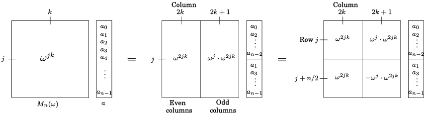
Figure FFT in Matrix Form
Unitary matrix
(Proposition.) The absolute value or magnitude of the eigenvalues of unitary matrix are 1.
Proof: Suppose \(Q\) is unitary matrix and \(Q v = \lambda v\),
\[\|v\|_2^2 = \langle Q v, Q v \rangle = \langle \lambda v, \lambda v \rangle = \bar{\lambda}\lambda \|v\|_2^2 = \vert \lambda \vert^2 \|v\|_2^2\]which concludes \(\vert \lambda \vert^2 = 1\). □
Remark. From its eigvalues we can see a unitary matrix only rotates or reflects a vector in \(\mathbb{C}\).
Hermitian and Spectral Theorem
(Definition.) Let \(V\) be a finite-dimensional vector space, and \(A: V \rightarrow V\) be a linear operator. The adjoint of \(A\) is the linear operator \(A^*: V \rightarrow V\) characterized by
\[\langle A^* v, w \rangle = \langle v, A w \rangle \quad \forall v, w \in V.\](Proposition.) The adjoint of \(A^*\) is \(A\).
Proof: By the definition of adjoint \(\langle A^{**} v, w \rangle = \langle v, A^{*} w \rangle\), thus it is sufficient to show \(\langle v, A^{*} w \rangle = \langle A v, w \rangle\).
\[\begin{aligned} \langle v, A^{*} w \rangle &= \overline{\langle A^{*} w, v \rangle} \quad \text{(conjugate symmetry)}\\ &= \overline{\langle w, A v \rangle} \quad (\text{definition of } A^*)\\ &= \langle A v, w \rangle. \end{aligned}\]Proof is completed. □
(Definition.) A linear operator \(A\) is called self-adjoint or Hermitian if \(A^* = A\).
(Proposition.) The eigenvalues of Hermtian are real and the eigenvectors corresponding to different eigenvalues are orthogonal.
Proof: Suppose \(v\) is the eigenvector corresponds to eigenvalue \(\lambda\),
\[\begin{aligned} \lambda \| v \|_2^2 &= \langle v, A v \rangle \\ &= \langle A v, v \rangle \quad (A \text{ is Hermitian})\\ &= \overline{\langle v, A v \rangle} \quad (\text{conjugate symmetry})\\ &= \overline{\lambda \| v \|_2^2} \\ &= \overline{\lambda} \| v \|_2^2, \end{aligned}\]thus we conclude \(\lambda\) is real.
Now suppose \(A v_1 = \lambda_1 v_1\), \(A v_2 = \lambda_2 v_2\), and \(\lambda_1 \ne \lambda_2\),
\[\begin{aligned} \lambda_1 \lambda_2 \langle v_1, v_2 \rangle &= \langle A v_1, A v_2 \rangle \\ &= \langle v_1, A^* A v_2 \rangle \\ &= \langle v_1, A^2 v_2 \rangle \\ &= \langle v_1, \lambda_2^2 v_2 \rangle \end{aligned} \\ \Rightarrow (\lambda_1 \lambda_2 - \lambda_2^2) \langle v_1, v_2 \rangle = 0 \Rightarrow \langle v_1, v_2 \rangle = 0.\]Proof is completed. □
(Spectral Theorem.) The Hermitian operator \(A\) has a complete set of orthonormal eigenvectors. Each eigenvalue is real.
Proof: ntu-note. □
Projector
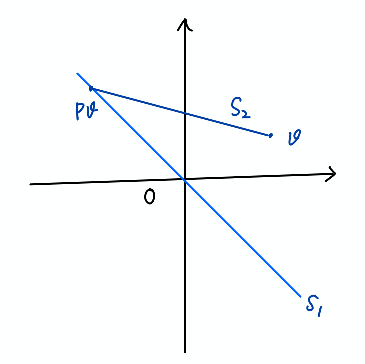
Figure Projector
(Proposition.) Suppose \(P\) is a projector that projects \(v\) onto \(P v\) along \((I-P)v\). Let \(S_1 = \{P v \mid v \in \mathbb{C}^m\}\) and \(S_2 = \{(I - P) v \mid v \in \mathbb{C}^m\}\). Then \(P\) seperates \(\mathbb{C}^m\) into two space \(S_1\) and \(S_2\) such that \(S_1 \bigcap S_2 = \{0\}\) and
\[\begin{aligned} S_1 &= \mathrm{range}(P) = \mathrm{null}(I - P),\\ S_2 &= \mathrm{range}(I - P) = \mathrm{null}(P). \end{aligned}\]Proof: We shall prove \(\mathrm{range}(I-P)=\mathrm{null}(P)\) as follows.
First, for any \(v \in \mathrm{null}(P)\) we have \(v = v - P v = (I-P)v \in \mathrm{range}(I-P)\). Hence, \(\mathrm{null}(P) \subseteq \mathrm{range}(I-P)\).
Next, for any \((I - P) v \in \mathrm{range}(I - P)\) we have \(P(I-P)v = (P - P^2) v = 0\). Thus, \(\mathrm{range}(I-P) \subseteq \mathrm{null}(P)\).
Now, by writing \(P = I - (I - P)\) we can obtain \(\mathrm{range}(P) = \mathrm{null}(I - P)\).
\(\mathrm{null}(P) \bigcap \mathrm{null}(I - P) = \{0\}\) because for any \(v \in \mathbb{C}^m\) in both of them satisfies
\[v = \underbrace{ v - P v}_{\text{in null}(P)} = \underbrace{ (I - P) v}_{\text{in null}(I - P)} = 0.\]Proof is completed. □
Remark. It should be pointed out that a projector projects the space onto a subspace. In the Figure Projector the hyperplane \(S_1\) is a subspace since it passes through origin.
(Proposition.) The eigenvalues of the projector is either 0 or 1.
Proof: Suppose \(P\) is a projector and let \(\lambda\) be its eigenvalue and \(v\) be the corresponding eigenvector then
\[\begin{array}{lll} P v &= \lambda v &\Rightarrow P^2 v &= \lambda P v \Rightarrow\\ P v &= \lambda^2 v &\Rightarrow \lambda v &= \lambda^2 v \end{array}\]If \(v \ne 0\) then \(\lambda = 0\) or \(\lambda = 1\). □
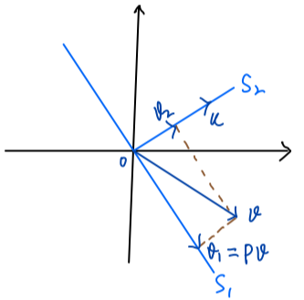
Figure Orthogonal Projector
(Orthogonal Projector.) An orthogonal projector projects the space onto a subspace \(S_1\) along a subspace \(S_2\), where \(S_1\) and \(S_2\) are orthogonal. Any projector that is hermitian is orthogonal projector.
\[v_2 = v - P v = (I - P) v \in \mathrm{range}(I - P) = \mathrm{null}(P) = S_2.\]For \(v_2 \in S_2\), \(P v_2 = 0\) since \(S_2 = \mathrm{null}(P)\).
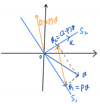
Figure Reflector
(Proposition.) If \(P\) is an orthogonal projector, \(I - 2P\) is a unitary matrix.
Proof: It is easy to verify \((I - 2P)(I - 2P)^* = I\). □
As the Figure Reflector shown \((I - 2P)v = (I - P)v - Pv = v_2 - v_1\), that is, \(I - 2P\) is a reflector. It is used to construct reflector in Householder QR Factorization.