Introduction to Differential Equations

Introduction to Differential Equations.

• Unit 1 Modeling and First Order ODEs
  • 1 Introduction to Differential Equations and Modeling
  • 2 Solving First Oder ODEs
    • Standard linear form
    • Conduction and diffusion
    • Solutions to homogeneous linear equations
    • Solutions to inhomogeneous linear equations
    • Superposition principle
    • Existence and uniqueness theorem for a linear ODE
    • Newton’s law of cooling down
• Unit 2: Complex Exponentials and ODEs
  • 3 Introduction to Complex Numbers
    • Polar form
    • Euler’s formula
    • Exponential law
    • Operations in polar form
  • 4 Complex Exponential Function
  • 5 Homogeneous 2nd Order Linear ODEs with Constant Coefficients
• Unit 3 Damped Oscillations
  • 6 Sinusoidal Functions
  • 7 Damped Harmonic Oscillators
    • Case 1: underdamped, \(b^2 < 4mk\)
    • Case 2: overdamped, \(b^2 > 4mk\)
    • Case 3: critically damped, \(b^2 = 4mk\)
    • Comparing damping qualitatively
    • Real life application: the rocking motion of a boat
  • 8 Higher Order Linear ODEs
• Unit 4 Exponential Response and Resonance
  • 9 Operator Notation
  • 10 Complex Replacement, Gain and Phase Lag, Stability
  • 11 Resonance, Frequency Response, RLC circuits
• Unit 5 Nonlinear DEs
  • 12 Nonlinear DEs: Graphical methods
  • 13 Autonomous equations
  • 14 Numerical Methods

Unit 1 Modeling and First Order ODEs

1 Introduction to Differential Equations and Modeling

1. Identify relevant quantities, both known and unknown, and give them symbols. Find the units for each.
2. Identify the independent variable(s). The other quantities will be functions of them, or constants. Often time is the only independent variable.
3. Write down equations expressing how the functions change in response to small changes in the independent variable(s). Also write down any “laws of nature” relating the variables. As a check, make sure that all summands in an equation have the same units.

Often simplifying assumptions need to be made; the challenge is to simplify the equations so that they can be solved but so that they still describe the real-world system well.

2 Solving First Oder ODEs

Standard linear form

Every first order linear ODE can be written in standard linear form as follows:

\[\displaystyle \text {Homogeneous: } \quad {\color{blue}{\dot{y}}} + p(t) \, {\color{blue}{y}} = 0\] \[\displaystyle \text {Inhomogeneous: } \quad {\color{blue}{\dot{y}}} + p(t) \, {\color{blue}{y}} = q(t)\]

Conduction and diffusion

We have a model called Newton Cooling law which gives us a differential equation model for temperature conduction or concentration diffusion as a first order ODE:

\[{\color{blue}{\dot{y}}} + k {\color{blue}{y}} = k {\color{orange}{x}} .\]

where \(x\) is the external temperature or concentration and \(y\) is the temperature or concentration of interest.

Solutions to homogeneous linear equations

All first order homogeneous equations can be solved using seperation of variables.

Solutions to inhomogeneous linear equations

Variation of parameters or Integrating factors.

Integrating factors. we start with a first order, linear, inhomogeneous ODE:

\[\dot{y} + p(t) y = q(t)\]

To find an integrating factor:

1. Find an antiderivative \(P(t)\) of \(p(t)\). The integrating factor is \(e^{P(t)}\).

2. Multiply both sides of the ODE by the integrating factor \(e^{P(t)}\).

   \[\displaystyle e^{P(t)} \dot{y} + e^{P(t)} p(t) \, y = \displaystyle q(t) e^{P(t)}\]

   We do this mulitplication because it is now possible to express the left side as the derivative of something:

   \[\displaystyle e^{P(t)} \dot{y}(t) + e^{P(t)} p(t) \, y(t) = \displaystyle \frac{d}{dt} \left( e^{P(t)} y(t) \right) .\]

   Now we can carry out the integration.

   \[\begin{aligned} \displaystyle \frac{d}{dt} \left( e^{P} y \right) &= q e^P \\ \displaystyle e^{P} y &= \displaystyle \int q e^{P} \, dt \\ \displaystyle y &= \displaystyle e^{-P} \int q e^{P} \, dt. \end{aligned}\]

   The indefinite integral \(\displaystyle \int q(t) e^{P(t)} \, dt\) represents a family of solutions because there is a constant of integration. If we fix one antiderivative, say \(R(t)\), then the others are \(R(t) + C\) for a constant \(C\). So the general solution is

   \[y = R(t) e^{-P(t)} + C e^{-P(t)}.\]

   Note that \(e^{-P}\) is the reciprocal of a solution to the homogeneous equation.

Superposition principle

1. \[\begin{aligned} \displaystyle \text {Multiplying a solution to}\quad p_ n(t) \, {\color{blue}{y^{(n)}}} + \cdots + p_0(t) \, {\color{blue}{y}} &= \displaystyle {\color{orange}{\phantom{a} q(t)}} \quad \text {by a number } {\color{orange}{a}} \\ \displaystyle \text {gives a solution to}\quad p_ n(t) \, {\color{blue}{y^{(n)}}} + \cdots + p_0(t) \, {\color{blue}{y}} &= \displaystyle {\color{orange}{a}} {\color{orange}{q(t)}} . \end{aligned}\]
2. \[\begin{aligned} \displaystyle \text {Adding a solution of }\quad p_ n(t) \, {\color{blue}{y^{(n)}}} + \cdots + p_0(t) \, {\color{blue}{y}} &= \displaystyle {\color{orange}{\phantom{a} q(t)}} \quad \text {by a number } {\color{orange}{a}}\\ \displaystyle \text {to a solution of}\quad p_ n(t) \, {\color{blue}{y^{(n)}}} + \cdots + p_0(t) \, {\color{blue}{y}} &= \displaystyle \quad \quad \quad {\color{orange}{q_2(t)}} \\ \displaystyle \text {gives a solution of}\quad p_ n(t) \, {\color{blue}{y^{(n)}}} + \cdots + p_0(t) \, {\color{blue}{y}} &= \displaystyle {\color{orange}{q_1(t)}} + {\color{orange}{q_2(t)}} . \end{aligned}\]

Existence and uniqueness theorem for a linear ODE

Let \(p(t)\) and \(q(t)\) be continuous function on an open interval \(I\). Let \(a \in I\), and let \(b\) be a given number. Then there exists a unique solution to the first order linear ODE

\[\dot y + p(t) \, y = q(t)\]

satisfying the initial condition

\[y(a)=b.\]

Newton’s law of cooling down

\[\frac{dT}{dt} = k (T_e - T)\]

\(k > 0\) is the conductivity and \(T_e\) is the external temperature. The solution is

\[T = T_e + (T_0 - T_e)e^{-kt}.\]

The general solution for the homogeneous equation \(dT/dt = kT\) is

\[T = ce^{kt}.\]

Unit 2: Complex Exponentials and ODEs

3 Introduction to Complex Numbers

Polar form

Fig.

To specify a preferred polar form, we would have to restrict the range for \(\theta\) to some interval of width \(2\pi\). The most common choice is to requrie \(-\pi < \theta \leq \pi\). This special \(\theta\) is called the principal value of the argument.

Given a complex number \(a + bi\) with \(a, b \neq 0\), how do we find the principal value of the argument \(\theta \in (-\pi, \pi]\)? There are two angles in \((-\pi, \pi]\) having tangent equal to \(b/a\), corresponding to opposite directions. By definition, \(\tan ^{-1}(b/a)\) is the one in \((-\pi /2,\pi /2)\). If \(a + bi\) is in the right half plane, then \(\theta = \tan ^{-1}(b/a)\) works. Otherwise, it is necesary to adjust \(\tan ^{-1}(b/a)\) by adding or subtracting \(\pi\).

Fig. Principal value of arctan

Euler’s formula

\[e^{i\theta }=\cos (\theta )+i\sin (\theta ).\] \[\textrm{For any constant }\, a, \, \, e^{at} \, \textrm{ is the solution of } \, \, \dot x=ax, \quad x(0)=1.\]

For \(z = re^{i\theta}\in \mathbb{C}\),

• adding an angle \(\theta_1 > 0\) to \(\theta\) is equivalent to rotating \(\theta\) by \(\theta_1\) counterclockwise;

• subtracting an angle \(\theta_1 > 0\) from \(\theta\) is equivalent to rotating \(\theta\) by \(\theta_1\) clockwise.

Exponential law

\[\begin{aligned} e^{i t_1} e^{i t_2} &= \displaystyle \left(\cos t_1 + i \sin t_1 \right)\left(\cos t_2 + i\sin t_2 \right) \\ &= \displaystyle \underbrace{ \left(\cos t_1\cos t_2 - \sin t_1\sin t_2 \right)}_{\cos (t_1+t_2)} + i \underbrace{\left(\sin t_1 \cos t_2 + \sin t_2 \cos t_1 \right)}_{\sin (t_1+t_2)} \\ &= \displaystyle \cos (t_1 + t_2) + i \sin (t_1+t_2) \\ &= \displaystyle e^{i(t_1+t_2)} \end{aligned}\]

\(e^{it}\) satisfies the initial value problem \(y' = i y\), \(y(0) = 1\).

\[\displaystyle \displaystyle \frac{d}{dt}e^{it} = \displaystyle ie^{it}.\]

Operations in polar form

Good for multiplication. We can write complex numbers \(z = a + bi\) in polar form as \(re^{i\theta } = r\cos (\theta ) + ir\sin (\theta ).\)

\[r_1 e^{i\theta _1} = r_2 e^{i \theta _2} \quad \textrm{if and only if}\quad r_1 = r_2 \; \textrm{ and }\; \theta _1 = \theta _2 + 2\pi k \textrm{ for some integer } k.\]

(This assumes that \(r_1\) and \(r_2\) are nonnegative real numbers, and that \(\theta_1\) and \(\theta_2\) are real numbers.)

Some arithmetic operations on complex numbers are easy in polar form:

\[\begin{array}{rl} \mathrm{multiplication}\qquad& \displaystyle (r_1 e^{i\theta _1})(r_2 e^{i\theta _2}) &=\quad \displaystyle r_1 r_2 e^{i(\theta _1 + \theta _2)} \\ \mathrm{reciprocal}\qquad& \displaystyle \frac{1}{r e^{i\theta }} &=\quad \displaystyle \frac{1}{r} e^{-i\theta } \\ \mathrm{division}\qquad& \displaystyle \frac{r_1 e^{i\theta _1}}{r_2 e^{i\theta _2}} &=\quad \displaystyle \frac{r_1}{r_2} e^{i(\theta _1 - \theta _2)} \\ n^{\textrm{th}} \textrm{ power}\qquad& \displaystyle (r e^{i\theta })^ n &=\quad \displaystyle (r e^{i\theta })^ n \\ \mathrm{complex\ conjugation}\qquad& \displaystyle \overline{r e^{i\theta }} &=\quad \displaystyle r e^{-i\theta } . \end{array}\]

Taking absolute values gives identies:

\[|z_1 z_2|=|z_1|\, |z_2|, \quad \left|\frac{1}{z}\right| = \frac{1}{|z|},\quad \left|\frac{z_1}{z_2}\right| = \frac{|z_1|}{|z_2|}, \quad |z^ n| = |z|^ n, \quad |\overline{z}| = |z|.\]

How do you trap a lion?

Fig. Trap a Lion

4 Complex Exponential Function

Fundamental Theorem of algebra. Every degree \(n\) complex polynomial \(f(z)\) has exactly \(n\) complex roots, if counted with multiplicity.

\[z^n = 1\]

since \(1 = e^{i (0 + 2k\pi)}\) for \(k \in \mathbb{Z}\), then \(z = e^{i (0 + 2k\pi)/n}\).

The \(n^\mathrm{th}\) roots of unity are the numbers \(e^{i \left( \frac{2\pi k}{n} \right)}\) for \(k=0,1,2,\ldots ,n-1\). Taking \(k=1\) gives the number \(\zeta \triangleq e^{2 \pi i/n}\). In terms of \(\zeta\), the complete list of \(n^{\mathrm{th}}\) roots of unity is

\[1, \; \zeta , \; \zeta ^2, \; \ldots , \; \zeta ^{n-1}\]

Geometrically, they all lie on the unit circle in the complex plane. The roots are evenly spaced around the unit circle, starting with the root $z = 1$, and the angle between two consecutive roots is \(2\pi/n\). These facts are illustrated for the case \(n=6\) in the figure below.

Fig. Roots of Unity

Analogously, we can find the \(n^\mathrm{th}\) roots of \(i\). As \(i = e^{i(\pi/2 + 2k\pi)}\) for \(k \in \mathbb{Z}\), so its \(n^\mathrm{th}\) roots have the form

\(e^{i(\pi/2 + 2k\pi)/n},\quad k = 0, 1, \ldots, n-1.\) Integration with complex number trick.

\[\begin{aligned} \int e^{2t} \cos(3t) dt &= \int \mathrm{Re}(e^{2t} e^{i3t}) dt \\ &= \mathrm{Re}\left(\int e^{2t} e^{i3t} dt\right) \end{aligned}\]

The second equality holds since only the real parts contribute to the real part of the sum in the summation of a series of complex numbers.

\[\begin{aligned} \int e^{2t} e^{i3t} dt &= \frac{1}{\sqrt{13}} e^{2t + (3t-\theta)i} + C \\ &= \frac{1}{13}e^{2t}(2\cos(3t) + 3\sin(3t)) + C \end{aligned}\]

where \(\theta = \arctan(3/2)\).

5 Homogeneous 2nd Order Linear ODEs with Constant Coefficients

Spring mass dashpot system. A mass sits on a cart is attched to a spring attached to a wall. The mass is also attached to a dashpot, a damping device. Finding the differential equation for the position of the mass.

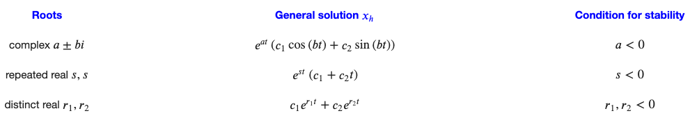
Fig. String Mass Dashpot

• \(F_{\mathrm{spring}}\) is a function of the position \(x\), and has opposite sign of \(x\);
• \(F_\mathrm{dashpot}\) is a function of velocity \(x'\), and has opposite sign of \(x'\).

\[F_\mathrm{spring} = -k x, \quad F_\mathrm{dashpot} = -bx',\]

Newton’s second law \(F = m x''\) gives

\[\displaystyle m \ddot{x} = -k x - b \dot{x},\]

a second linear ODE, which we usually write as

\[m {\color{blue}{\ddot{x}}} + b {\color{blue}{\dot{x}}} + k {\color{blue}{x}} =0.\]

Solution: Try \(x = e^{rt}\), where \(r\) is a constant to be determined. Substituting it to the above equation,

\[\begin{aligned} \displaystyle mr^2 e^{rt} + b r e^{rt} +k e^{rt} &= 0\\ \displaystyle (mr^2 + br +k) e^{rt} &= 0 \end{aligned}\]

The polynomial \(p(r)\, =\, mr^2 + br +k\) is known as the characteristic polynomial of the given DE, and the equation \(p(r) = 0\) is the characteristic equation.

Suppose that the characteristic equation has two real roots \(r_1, r_2\). The solution of the original DE will be

\[x(t) = c_1 e^{-r_1 t} + c_2 e^{-r_2 t}.\]

Suppose that the equation \(\ddot y + A\dot y + By = 0\,\) where \(A, B\) are real, has characteristic roots \(a \pm ib\). Then the general real solution is

\[\begin{aligned} y(t) &= c_1 e^{(a+ib)t} + c_2 e^{(a - ib)t}\\ \quad \text{or} \\ y(t) &= \displaystyle c_1e^{at}\cos (bt) + c_2 e^{at}\sin (bt). \end{aligned}\]

This is due to if \(\, y(t)=u(t)+iv(t)\,\) is a solution to a second order homogeneous linear DE with real coefficients: \(\displaystyle \ddot{y} + A\dot{y}+By = 0\). Then

\[\displaystyle \left( \ddot u+A \dot u+ Bu\right) +i \left( \ddot v+A \dot v+ Bv\right) = 0\]

which implies both \(u\) and \(v\) are solutions to the original DE.

In particular, the general solution represented by \(m, b, k\) is

\[x(t) = \displaystyle e^{(-b/2m)t} \left( c_1\cos \left(\omega _ d t\right)+c_2 \sin \left(\omega _ d t\right)\right) \qquad c_1,\, c_2 \in \mathbb {R},\]

where \(\, \displaystyle \omega _ d\, =\, \sqrt {\frac{k}{m}-\frac{b^2}{4m^2}}\,\).

Unit 3 Damped Oscillations

6 Sinusoidal Functions

Recall the spring-mass-dashpot system with no external force, when there are two distinct characteristic complex roots, the general real solution:

\[x(t) = \displaystyle e^{(-b/2m)t} \left( c_1\cos \left(\omega _ d t\right)+c_2 \sin \left(\omega _ d t\right)\right) \qquad c_1,\, c_2 \in \mathbb {R},\]

where \(\, \displaystyle \omega _ d\, =\, \sqrt {\frac{k}{m}-\frac{b^2}{4m^2}}\,\) is called the damped frequency of the system.

Fig.

If the system has no damping, the DE reduces to

\[m {\color{blue}{\ddot{x}}} + k {\color{blue}{x}} =0\qquad m, k>0,\]

and the general solution reduces to

\[x(t) = \displaystyle c_1 \cos \left(\omega _ n t\right)+c_2\sin \left(\omega _ n t\right) \qquad c_1,\, c_2 \in \mathbb {R},\]

where \(\, \displaystyle \omega _ n\, =\, \sqrt {\frac{k}{m}}\,\) is called the natural frequency of the system. Note that \(\omega_n > \omega_d\), this coincides with our intuition that the cart should oscillate more frequently when no damping.

\[\begin{aligned} \displaystyle \displaystyle \underbrace{\color{blue}{a} \cos (\theta )+{\color{blue}{b}}\sin(\theta)}_{\color{blue}{\text{rectangular form}}}\, &= \displaystyle \underbrace{\color{orange}{A} \cos (\theta -{\color{orange}{\phi }} )}_{\color{orange}{\text {polar form}}}\qquad {\color{blue}{a}} ,\, {\color{blue}{b}} ,\, {\color{orange}{\phi }} \in \mathbb {R}, \ \ \ {\color{orange}{A}} \geq 0 \in \mathbb {R}, \\ &= \displaystyle \underbrace{\color{orange}{A} \cos {\color{orange}{\phi }}}_{\color{blue}{a}} \cos \theta + \underbrace{\color{orange}{A} \sin {\color{orange}{\phi }} }_{\color{blue}{b}} \sin \theta \qquad \text {by the trig sum formula} \end{aligned}\]

where \(A, \phi\) in terms of \(a, b\) are given implicitly by the following diagram:

Fig.

As usual, the angle \(\phi\) is well-defined only up to addition of integer multiples of \(2\pi\).

Proof:

1. Using complex numbers. Let us write \(c = a - bi\), as a consequence,

   \[\mathrm{Re}(c(\cos(\theta) + i \sin(\theta))) = a\cos(\theta) + b\sin(\theta).\]

   On the other hand, \(c = Ae^{-i\phi}\) and \(\cos(\theta) + i \sin(\theta) = e^{i\theta}\),

   \[\mathrm{Re}(c(\cos(\theta) + i \sin(\theta))) = \mathrm{Re}(Ae^{-i\phi} e^{i\theta}) = A \cos(\theta - \phi).\]

2. The geometric perspective. Let us consider \(a\cos(\theta) + b\sin(\theta)\) as the inner product of two vectors \(\mathbf{x} = [a, b]\) and \(\mathbf{y} = [\cos(\theta), \sin(\theta)]\), since

   \[\langle \mathbf{x}, \mathbf{y} \rangle = \|\mathbf{x}\|_2 \|\mathbf{y}\|_2 \cos(\mathrm{angle\ between\ } \mathbf{x}\ \mathrm{and}\ \mathbf{y}) = A \cos(\phi - \theta).\]

Graphing sinusoidal functions

Fig. Sinusoidal Functions

\[f(t)=A \cos (\omega t-\phi )\]

• \(A\), amplitude.

• \(P\), period, the time for one complete oscillation.

• \(\omega = \frac{2\pi}{P}\) (radians/second) is called angular frequency or circular frequency; there is also frequency \(\nu = \frac{1}{P}\) (Hertz = cycles per second), the number of complete oscillations per second.
• \(\phi\) (radians), phase lag or phase shift.

7 Damped Harmonic Oscillators

no damping. DE: \(\displaystyle m \ddot{x} + k x = 0 \qquad (m, k > 0)\).

This system or any other system governed by the same DE, is called simple harmonic oscillator. The angular frequency \(\omega_n = \sqrt{\frac{k}{m}}\) is called natural frequency or resonant frequency of the oscillator.

damping. DE: \(\displaystyle m \ddot{x} + b \dot{x} + k x = 0 \qquad (m, c, k > 0)\). Now we rewrite it as

\[\begin{aligned} \ddot{x} + \frac{b}{m} \dot{x} + \frac{k}{m} x &= 0 \\ \ddot{y} + 2p \dot{y} + \omega_n^2 &= 0 \end{aligned}\]

Case 1: underdamped, \(b^2 < 4mk\)

The real part is \(-p = -\frac{b}{2m}\). The imaginary part is either positive or negative of the damped frequency \(\omega_d\),

\[\begin{aligned} {\color{blue}\omega_d} &\triangleq \displaystyle {\color{blue}{\frac{\sqrt {4mk-b^2}}{2m}}}\\ &= \displaystyle {\color{blue}{\sqrt{\omega_n^2-p^2}}} \ ,\qquad \text {where } \, {\color{blue}{\omega_n=\sqrt{\frac{k}{m}}}} \, \, \text {is the natural frequency}. \end{aligned}\]

Sumary of results:

\[\begin{aligned} \mathrm{Roots}:&\qquad \, \, \displaystyle - p\pm i\omega _ d \\ \mathrm{Basis\ of\ solution\ space}:&\qquad e^{(-p + i\omega _ d)t}, \; e^{(-p - i\omega _ d)t}\\ \mathrm{Real\ valued\ basis}:&\qquad e^{-p t} \cos (\omega _ d t), \; e^{-p t} \sin (\omega _ d t)\\ \mathrm{General\ real\ solution}:&\qquad {\color{blue}{e^{-p t} (a \cos (\omega _ d t) + b \sin (\omega _ d t))}}, \mathrm{where\ }a, b \mathrm{\ are\ real\ constants}\\ &\qquad = {\color{blue}{A e^{-pt}\cos (\omega _ d t - \phi )}} \end{aligned}\]

Note that \(\omega_d\) depends on the spring (\(k\)) and dashpot (\(b\)), whereas \(A, \phi\) only depends on the inital conditions.

Case 2: overdamped, \(b^2 > 4mk\)

The roots \(\, \displaystyle \frac{-b \pm \sqrt {b^2-4mk}}{2m}\,\) are real and distinct. Both roots are negative, since \(\sqrt{b^2 - 4mk} < b\). Call them \(-s_1\) and \(-s_2\), and assume that \(-s_1 > -s_2\). General solution:

\[{\color{blue}{a e^{-s_1 t} + b e^{-s_2 t}}}, \mathrm{where\ }a, b \mathrm{\ are\ real\ constants}.\]

All solutions tend to \(0\) as \(t \to +\infty\). The first term eventually controls the rate of return to equilibrium.

Case 3: critically damped, \(b^2 = 4mk\)

\[\begin{aligned} \mathrm{Basis\ of\ solution\ space}:&\qquad e^{-pt}, \; te^{-pt}\\ \mathrm{General\ real\ solution}:&\qquad {\color{blue}{e^{-pt} (a + b t)}}, \mathrm{where\ }a, b \mathrm{\ are\ real\ constants}\\ \end{aligned}\]

Since the second order equation must have two distinct special solutions, we can assume its solution takes the form \(e^{-pt} u\) and apply variation of parameters to get \(t e^{-pt}\).

Comparing damping qualitatively

Consier the DE \(\ddot{x}+b\dot{x}+x= 0\) with initial conditions \(x(0)=1\), \(\dot x(0) = 0\). We will consider the three cases \(b=1, 2, 3\),

\[\begin{aligned} x_1(t) \displaystyle &=e^{-t/2}\left(\cos \frac{t\sqrt {3}}{2}+\frac{1}{\sqrt {3}}\sin \frac{t\sqrt {3}}{2}\right),\\ \displaystyle {\color{blue}{x_2(t)}} \displaystyle &=e^{-t}\left(1+t\right), \\ \displaystyle {\color{orange}{x_3(t)}} \displaystyle &=\left(\frac{1}{2}+\frac{3}{2\sqrt {5}}\right)e^{\frac{-3+\sqrt {5}}{2}t}+\left(\frac{1}{2}-\frac{3}{2\sqrt {5}}\right)e^{\frac{-3-\sqrt {5}}{2}t}. \end{aligned}\]

shown in the below figure, from which we can conclude that the smaller \(b\) the faster the mass moves to the equilibrium position at the first round.

Fig.

Real life application: the rocking motion of a boat

Fig. Rocking Motion of a Boat

The rotational motion of a boat rocking sideways close to its flat equilibrium position is described by the linear approximation of the rotational version of Newton’s second law:

\[\displaystyle I \ddot{\theta } = \displaystyle \tau (\theta ) \qquad \text {where} \, \tau (\theta )\, \text {is the torque}\]

where \(I > 0\) is the moment of inertia of the boat, \(\tau\) is the torque exerted on the boat and when \(\theta\) is small \(\tau\) can be approximated as a linear function of \(\theta\)

\[\tau(\theta) = \displaystyle -k \theta \qquad \text {where }\, k>0, \, \theta \ll 1.\]

\(I\) and \(k\) are constants determined by the geometry and distribution of mass of the boat. The differential equation describes the motion is

\[I \ddot{\theta } + k \theta = 0\]

Since \(I > 0, k > 0\) the boat will do harmonic oscillation. But if the boat is not well designed, \(k\) can be negative in which case the differential equation solution becomes (assume \(\, \theta (0)=0,\, \dot\theta (0)=c\))

\[\theta(t) = \frac{c}{2} \sqrt{\frac{I}{k}} e^{\sqrt{k/I} t} - \frac{c}{2} \sqrt{\frac{I}{k}} e^{-\sqrt{k/I} t},\]

from which we can see that the boat will capsize.

The centroid of a shape on the plane is the average position of all points of the shape.

8 Higher Order Linear ODEs

Given

\[a_ n {\color{blue}{y^{(n)}}} + \cdots + a_1 {\color{blue}{\dot{y}}} + a_0 {\color{blue}{y}} = 0,\]

where \(a_i\) are real constants, do the following:

1. Write down the characteristic equation

   \[a_ n r^ n + \cdots + a_1 r + a_0 = 0.\]

2. Factor \(P(r)\) as

   \[P(r)\, =\, a_ n (r-r_1)(r-r_2)\cdots (r-r_ n)\]

   There are guaranteed to be \(n\) (complex) roots counted with multiplicity by the fundamental theorem of algebra.

3. If \(\, r_1,\ldots ,r_ n\,\) are distinct, then the functions \(\, e^{r_1 t},\ldots ,e^{r_ n t}\,\) form a basis for the vector space of solutions to the constant coefficient ODE, the general solution is

   \[c_1 e^{r_1 t} + \cdots + c_ n e^{r_ n t}.\]

   Note that complex roots always appear in pairs of conjugates, and if some of the roots are complex, the coefficients \(c_i\) will have to be complex as well.

4. If a particular root \(r\) is repeated \(m\) times, then

   replace \(\displaystyle \overbrace{e^{rt},\quad e^{rt},\quad e^{rt},\quad \ldots ,\quad e^{rt}}^{\color{orange}{m \textrm{ copies}}}\) by \(\displaystyle e^{rt},\quad te^{rt},\quad t^2 e^{rt},\quad \ldots ,\quad t^{m-1} e^{rt}.\)

Example 1: Find a basis of solutions to \(y^{(3)} + 3 \ddot{y} + 9 \dot{y} - 13 y = 0\) consisting of real-valued functions.

The characteristic polynomial is \(\, P(r) \colon =r^3+3r^2+9r-13 = (r-1)(r^2+4r+13).\, \,\) Rewriting the second factor as \((r+2)^2 + 9\), shows that the roots of \(P(r)\) are \(1, -2+3i, -2-3i\). Thus \(e^t, e^{(-2+3i)t}, e^{(-2-3i)t}\) form a basis of solutions. But the last two are not real-valued, instead

\[\displaystyle e^{(-2+3i)t} \displaystyle = e^{-2t} \cos (3t) + i \, e^{-2t} \sin (3t).\]

Thus

\[{\color{blue}{e^ t,\quad e^{-2t} \cos (3t), \quad e^{-2t} \sin (3t)}}\]

is another basis.

Example 2: Suppose the roots with multiplicity of the characteristic polynomial of a certain homogeneous constant coefficient linear equation are

\(3, 4, 4, 4, 5, 5 \pm 2i, 5 \pm 2i.\) what is the general real solution to the equation.

A basis for the real-valued solutions is given by

\(\{ e^{3t}, \, e^{4t}, \, te^{4t}, \, t^2e^{4t}, \, e^{5t}\cos (2t), \, e^{5t}\sin (2t), \, te^{5t}\cos (2t), \, te^{5t}\sin (2t)\} .\) Using superposition, the general solution is a linear combination of these basis solutions

\[\begin{aligned} x(t) = \displaystyle \, &c_1e^{3t}+ c_2e^{4t}+c_3te^{4t} +c_4t^2e^{4t} \\ &\displaystyle + c_5e^{5t}\cos (2t)+c_6 e^{5t}\sin (2t) + c_7te^{5t}\cos (2t) + c_8 te^{5t}\sin (2t). \end{aligned}\]

Unit 4 Exponential Response and Resonance

9 Operator Notation

An operator takes an input function and returns another function.

In general, a linear operator \(L\) is any operator that satisfies

\[L(f+g) = Lf + Lg, \qquad L(af) = a\, Lf\]

for any functions \(f\) and \(g\), and any number \(a\).

Polynomial differential operators with constant coefficients,

\[\displaystyle P\left(D\right)=a_ nD^ n+a_{n-1}D^{n-1}+\dots a_1D+a_0,\]

where all of the coefficients \(a_k\) are numbers. All operators of this form are linear. In addition to being linear operators, they are also time invariant operators, which means: If \(x(t)\) solves \(P(D)x = f(t)\), then \(y(t) = x(t-t_0)\) solves \(P(D) y = f(t-t_0)\).

Since \(P(D)x(t) = f(t)\) holds for any \(t\) and \(P(D)\) does not involve \(t\) (constant coefficients), we simply replace \(t\) with \(t- t_0\) in the equation to obtain \(P(D)x(t-t_0) = f(t-t_0)\).

A system that can be modeled using a linear time invariant operator is called an LTI (linear time invariant) system.

Example. The function \(x(t) = \sin (t)\) solves the differential equation \(\dot x = \cos t\). what is a solution to the differential equation \(\dot y = \cos (t +\pi /2)\)? By time invariant, one solution is \(y=\sin (t+\pi /2)\).

Example. Consider the differential equation \(\displaystyle \dot{x}+x=\cos t\). Variation of parameters or integrating factors tells us that the general solution to this differential equation is

\[\displaystyle x\left(t\right)=\frac12\cos t + \frac12 \sin t+c_1e^{-t}.\]

Now suppose we want to solve the equation \(\dot{y}+y=\sin t\). Since \(\sin t=\cos \left(t-\pi /2\right)\), time invariance tells us that

\[\begin{aligned} \displaystyle y\left(t\right) &= \displaystyle x\left(t-\frac{\pi }{2}\right)=\frac12\cos \left(t-\pi /2\right) + \frac12 \sin \left(t-\pi /2\right)+c_1e^{-\left(t-\pi /2\right)} \\ &= \frac12\sin \left(t\right) - \frac12 \cos \left(t\right)+c_2e^{-t} \end{aligned}\]

should solve \(\dot{y}+y=\sin t\).

Fig.

\[\text {inhomogeneous equation:} \quad p_ n(t) \, {\color{blue}{y^{(n)}}} + \cdots + p_0(t) \, {\color{blue}{y}} = {\color{orange}{q(t)}},\]

\(\text {homogeneous equation:} \quad p_ n(t) \, {\color{blue}{y^{(n)}}} + \cdots + p_0(t) \, {\color{blue}{y}} = 0;\) write down the general homogeneous solution \(y_h\).

\[\underset {\color{blue}{\text{general solution}}}{y} = \underset{\color{blue}{\text {particular solution}}}{y_p} + \underset {\text {general homogeneous solution}}{y_h}.\]

Let \(L\) be the linear operator \(L = p_ n(t)D^ n + \dotsb + p_1(t)D+p_0(t)\). Then the differential equations become

\[\begin{aligned} \displaystyle \text {inhomogeneous equation} \qquad Ly &= q(t) \\ \displaystyle \text {homogeneous equation} \qquad Ly &= 0 \end{aligned}\]

we can prove that \(L(y_ p+y_ h) =q+0=q.\)

For any polynomial \(P\) and any number \(r\),

\({\color{blue}{P(D) e^{rt} = P(r) e^{rt}.}}\) For any polynomial \(P\) and number \(r\), what is a particular solution to \(P(D)y = e^{rt}?\)$

We have

\[P(D) {\color{blue}{e^{rt}}} = {\color{orange}{P(r) e^{rt}}} .\]

hence

\[P(D)\left(\frac{1}{P(r)}e^{rt} \right) = e^{rt}.\]

This is called Exponential Response Formula (ERF). In other words, for any polynomial \(P\) and number \(r\) such that \(P(r) \ne 0,\)

\[{\color{blue}{\frac{1}{P(r)} e^{rt}}} \quad \text { is a particular solution to }\quad P(D) y = {\color{blue}{e^{rt}}} .\]

Remark: \(P(D)\) is a linear operator, giving it a function \(e^{rt}\) it yields another function \(P(r)e^{rt}\).

Example. Find the particular solution to \(\ddot{y} + 7\dot{y} + 12 y = {\color{blue}{-5e^{2t}}}\).

ERF says

\[{\color{blue}{\frac{1}{P(2)} e^{2t}}} = {\color{blue}{\frac{1}{30} e^{2t}}} \quad \text {is a particular solution to }\quad P(D) y = {\color{blue}{e^{2t}}} ;\]

so

\[\underset {\color{blue}{\text {call this }y_p}}{-\frac{1}{6} e^{2t}} \quad \textrm{ is a particular solution to }\quad \ddot{y} + 7 \dot{y} + 12 y = {\color{blue}{-5e^{2t}}} .\]

The existence and uniqueness theorem syas that

\[P(D) y = e^{rt}\]

should have a solution even if \(P(r) = 0\) (when ERF does not apply).

ERF’ Suppose that \(P\) is a polynomial and \(P(r_0) = 0\), but \(P'(r_0) \neq 0\) for some number \(r_0\). Then

\[\boxed {\color{blue}{x_ p=\frac{1}{P'(r_0)} t e^{r_0t}} \quad \text { is a particular solution to }\quad P(D) x = {\color{blue}{e^{r_0t}}}.}\]

proof. We know that \(P(D)e^{rt} = P(r)e^{rt},\)

for all \(r\), so in particular \(P(D)e^{r_0t} = P(r_0)e^{r_0t}\). Since \(P(r_0) = 0\), we cannot divide it. Instead, we look at what happens for \(r\) near \(r_0\) by differentiating with respect to \(r\),

\[\displaystyle \displaystyle \frac{\partial }{\partial r}\left(P(D) e^{rt} \right) = \displaystyle \frac{\partial }{\partial r}\left(P(r) e^{rt} \right) = P'(r)e^{rt} + P(r)te^{rt}.\]

On the other hand, we can exchange the order of differentiation operator

\[\frac{\partial }{\partial r}D = D\frac{\partial }{\partial r} \qquad \left(D = \frac{d}{dt} \right).\]

Hence, by linearity of \(D\)

\[\frac{\partial }{\partial r}P(D) = P(D)\frac{\partial }{\partial r}.\]

The left hand side becomes,

\[\displaystyle \displaystyle \frac{\partial }{\partial r}\left(P(D) e^{rt} \right) = \displaystyle P(D) \left( \frac{\partial }{\partial r} e^{rt}\right) = \displaystyle P(D) \left( te^{rt}\right).\]

Let \(r \rightarrow r_0\),

\[\displaystyle P(D) \left( te^{r_0t}\right) = \displaystyle P'(r_0)e^{r_0t} + P(r_0)te^{r_0t} = \displaystyle P'(r_0)e^{r_0t}.\]

If \(P^{\prime}(r_0) \neq 0\), then we get

\[P(D) \left( \frac{te^{r_0t}}{P'(r_0)}\right) = e^{r_0t},\]

and \(\displaystyle y_ p = \frac{te^{r_0t}}{P'(r_0)}\) is a particular solution to \(P(D)y = e^{r_0t}\).

$\square$$

Generalized Exponential Response Formular. If \(P\) is a polynomial and \(r_0\) is a number that

\[P(r_0) = P'(r_0) = \dotsb = P^{(m-1)}(r_0) = 0 \qquad P^{(m)}(r_0) \neq 0,\]

then

\[P(D)\left( t^ me^{r_0t} \right) = P^{(m)}(r_0)e^{r_0t}\]

and

\[\boxed {\color{blue}{y_ p=\frac{1}{P^{(m)}(r_0)} t^ m e^{r_0t}} \quad \text { is a particular solution to }\quad P(D) y = {\color{blue}{e^{r_0t}}} .}\]

Example. Find a particular solution to \(\ddot x - 4x = e^{-2t}\).

Solution: \(P(r) = r^2 - 4\), and \(P(-2) = 0\). But \(P'(-2) = -4\). Therefore, we can apply ERF’, which gives us a particular solution

\[x_ p = \frac{te^{rt}}{P'(r)} = \frac{te^{-2t}}{-4}.\]

Revisiting basis of homogeneous solutions with linear operators. To know that \(e^{2t}\), \(e^{3t}\), \(e^{5t}\) really form a basis, we need to know that they are linearly independent. Could it instead be that

\[e^{5t} = c_1 e^{2t} + c_2 e^{3t} \qquad \text {(as functions)}\]

for some numbers \(c_1, c_2\)?

Applying the operator \((D-2)(D-3)\) to both sides, which would give

\[\begin{aligned} \displaystyle \displaystyle (D-2)(D-3)e^{5t} &= \displaystyle (D-2)(D-3)\left( c_1 e^{2t} + c_2 e^{3t} \right)\\ &= \displaystyle c_1(D-2)(D-3)e^{2t} + c_2 (D-2)(D-3) e^{3t} \qquad \text {(by linearity)}\\ &= 0 \end{aligned}\]

The left hand side gives us

\[(D-2)(D-3)e^{5t} = (5-2)(5-3) e^{5t} \neq 0.\]

This contradition implies that \(e^{5t}\) is not a linear combination of \(e^{2t}\) and \(e^{3t}\).

Remark: The key part is to note that \(P(D) := (D-2)(D-3)\) and \(P(D)e^{rt} = P(r)e^{rt}\).

Example. Find a basis of solutions to \((D-5)^3 y = 0\).

Solution. What does \((D-5)\) do to \(ue^{5t}\), if \(u\) is a function of \(t\)? Using the product rule:

\[\begin{aligned} (D-5) \, u e^{5t} &= \left( \dot{u}\cdot e^{5t} + u \cdot 5 e^{5t} \right) - 5 u \cdot e^{5t}\\ &= \dot{u} \cdot e^{5t}. \end{aligned}\]

Replacing \((D-5)\) by \((D-5)^k\) on the left we get \((D-5)^k u e^{5t} = u^{(k)} e^{5t}\). Hence, in oder for \(ue^{5t}\) to be a solution to \((D-5)^3 y=0\) the function \(u^{(3)}\) must be \(0\), i.e., \(u = a + b t + c t^2\) for some \(a, b, c\), so the solutions are

\[\displaystyle u e^{5t} = a \, e^{5t} + b \, t e^{5t} + c \, t^2 e^{5t}.\]

If a characteristic polynomial \(P(r)\) has a root \(r_0\) is repeated \(k\) times, then \(e^{r_0t}\), \(te^{r_0t}\), \(t^2 e^{r_0t}\), \(\ldots\), \(t^{k-1}e^{r_0t}\) are independent solutions to the differential equation \(P(D)y = 0\).

10 Complex Replacement, Gain and Phase Lag, Stability

Complex replacement is a method for finding a particular solution to an inhomogeneous linear ODE

\[P(D) x = {\color{orange}{\cos \omega t}} ,\]

where \(P\) is a real polynomial, and \(\omega\) is a real number.

1. Write the right hand side as \(\mathrm{Re}(e^{i \omega t})\):

   \[P(D)x = {\color{orange}{\mathrm{Re\, }\left( e^{i\omega t}\right)}} .\]

2. Replace the right hand side of differential equation with \(e^{i \omega t}\) and \(x\) with \(z\). The complexified differential equation is:

   \[P(D) {\color{blue}{z}} = \underset {\color{blue}{\text {complex replacement}}}{\color{blue}{e^{i\omega t}}.}\]

3. Use ERF to find a particular solution \(z_p\) to the complexified ODE:

   \[z_ p = \frac{e^{i\omega t}}{P(i\omega)}.\]

4. Compute \(x_p = \mathrm{Re}(z_p)\). Then \(x_p\) is a particular solution to the original ODE.

Example: Find a solution to \(\ddot{x} + 2x = e^{-t}\cos (3t - \phi )\) where \(\phi\) is a real number.

Replace the right hand side with

\[e^{-t} e^{i(3t - \phi)} = e^{-i \phi} e^{(3i-1)t}.\]

The complexified equation is

\[\displaystyle \displaystyle \ddot{z} + 2z\displaystyle = e^{-i\phi }e^{(-1+3i)t}.\]

Apply ERF with the characteristic polynomial \(P(r) = r^2 + 2\),

\[\displaystyle P(-1+3i) = \displaystyle (-1+3i)^2 + 2 = -6-6i,\]

and the complex solution is

\[z_ p = \frac{e^{-i\phi }e^{(-1+3i)t}}{-6 - 6i} = \frac1{6\sqrt {2}}e^{-i\phi +i3\pi /4}e^{(-1+3i)t}.\]

and

\[x_p = \displaystyle \mathrm{Re\, }(z_ p)= \frac1{6\sqrt {2}}e^{-t}\cos (3t-\phi + 3\pi /4).\]

We have an LTI system modeled by the differential equation

\[P(D) x = Q(D) y\]

with input signal \(y\) (e.g. ocean tide) and system response \(x\) (e.g. harbor water level). The ERF with complex replacement shows that if \(y = \cos(\omega t)\), then a particular solution is given by

\[x_ p = \mathrm{Re\, }\left(G(\omega )e^{i\omega t}\right) = g\cos (\omega t - \phi )\]

where (note that \(Q(D) e^{i \omega t}= Q(i \omega) e^{i \omega t}\))

\[G(\omega ) = \frac{Q(i\omega )}{P(i\omega )} \quad \text {if } P(i\omega ) \neq 0.\]

In general, we have

\[\begin{aligned} \mathrm{complex\ gain} &= G = \frac{x}{y} = \frac{Q(i\omega )}{P(i\omega )},\\ \mathrm{phase\ lag} &= -\arg G = \arg P(i\omega) - \arg Q(i\omega). \end{aligned}\]

If we know that \(x_ p = g\cos (\omega t - \phi )\) is a steady response to \(P(D) x = \cos (\omega t)\) then by LTI \(Ag\cos(\omega t - \theta - \phi)\) is a steady state response to \(P(D) x = A\cos (\omega t-\theta )\).

By time invariant (the system parameters are not changing over time), if \(x(t)\) is a system response to the input signal \(f(t)\), then \(x(t-t_0)\) is a system response to the input \(f(t-t_0)\); by linearity, if \(x(t)\) is a system response to \(f(t)\), then \(Ax(t)\) is a system response to \(Af(t)\). Thus study the input \(\cos(\omega t)\) is enough to yield solution of input \(A\cos(\omega t - \phi)\) for a linear time-invariant system.

Consider a LTI ODE

\[\ddot x + 7\dot x+12 x = 12f(t)\]

where \(f(t) = \cos(2t)\) is the input signal.

The general homogeneous solution has the form

\[x_ h = c_1 e^{-3t} + c_2 e^{-4t},\]

where \(c_1\) and \(c_2\) are constants. The general solution to the original ODE is

\[x = x_p + x_h = \underbrace{\mathrm{Re\, }\left( \frac{12}{8+14i} e^{2it} \right)}_{\color{blue}{\text {steady state solution}}} + \underbrace{c_1 e^{-3t} + c_2 e^{-4t}}_{\color{orange}{\text {transient}}}.\]

No matter what the initial conditions are, the transient vanishes as time goes to infinity.

A constant coefficient linear ODE of any order is stable if and only if every root of the characteristic polynomial has negative real part.

Fig.

11 Resonance, Frequency Response, RLC circuits

Example: We try to model a swing on a playground as a simple harmonic oscillator with natural frequency \(\omega_n\). When we push the swing, we give the system an input signal. Let’s model the system by a sinusoidally driven harmonic oscillator,

\[\ddot{x}+\omega _ n^2x=A\cos (\omega t)\]

We find a periodic solution using ERF provided that \(\omega \neq \omega_n\):

\[x_p = \displaystyle A\frac{\cos (\omega t)}{\omega _ n^2-\omega ^2}.\]

Remark: The output signal \(x_p\) has the same frequency as the input signal and the only change is the amplitude \(g := \frac{A}{\omega_n^2 - \omega^2}\). As \(\omega\) gets closer to \(\omega_n\), the amplitude \(g\) grows larger.

If \(\omega = \omega_n\) we can apply ERF’ to find a particular solution

\[x_p = \frac{t\sin (\omega _ n t)}{2\omega _ n}.\]

The response is an oscillating function whose oscillations grow linearly without bound as time increases.

Pure resonance is a phenomenon that occurs when a harmonic oscillator is driven with an input sinusoid whose frequency is at the natural frequency:

• the gain becomes larger and larger as the input frequency approaches the natural frequency, and
• when the input frequency equals the natural frequency, any particular solution is unbounded.

For the spring-mass-dashpot system, we use the notation

\[m\ddot x + b\dot x + kx = f_1(t)\]

and rewrite this as

\[\ddot x + 2p \dot x + \omega _ n^2 x = f_2(t)\]

by dividing through by \(m\):

\[\begin{aligned} 2p &= \frac{b}{m},\\ \omega_n^2 &= \frac{k}{m}. \end{aligned}\]

Suppose \(f_2(t) = A \cos(\omega t)\) then

\[|G(\omega)| = \frac{1}{|P(i\omega)|}\]

where \(P(i\omega) = -\omega^2 + 2p\omega i + \omega_n^2.\)

Let \(L(\omega^2) := \vert P(i\omega) \vert^2 = (\omega_n^2 - \omega^2)^2 + 4p^2 \omega^2\) and we have \(\frac{dL}{d\omega^2} = -2\omega^2_n + 2\omega^2 + 4p^2\) and \(L(\omega^2)\) is convex since its Hessian matrix is 2. Thus,

• \(\vert G(\omega^2) \vert\) achieves its maximum at \(\omega = \sqrt{\omega_n^2 - 2p^2}\), if \(\omega_n^2 - 2p^2 > 0\);
• \(\vert G(\omega^2) \vert\) is monotoneously decreasing, otherwise (since \(dL/d\omega^2 > 0\)).

RLC circuits.

Fig. RLC Circuits

\(R\) resistance of the resistor (ohms)

\(L\) inductance of the inductor (henries)

\(C\) capacitance of the capacitor (farads)

\(V\) voltage source (volts)

The quantities \(R, L, C\) are constants while the voltage source $V$$ is a function of time.

\[\begin{aligned} \displaystyle \displaystyle \text {Voltage drop across the }{\color{blue}{\text {inductor:}}}\quad & \displaystyle {\color{blue}{V_ L(t)}} =L\dot I(t). \\ \displaystyle \text {Voltage drop across the }{\color{blue}{\text {resistor:}}}\quad & \displaystyle {\color{blue}{V_ R(t)}} =RI(t). \\ \displaystyle \text {Voltage drop across the }{\color{blue}{\text {capacitor:}}}\quad & \displaystyle C {\color{blue}{\dot{V}_ C(t)}} = I(t). \end{aligned}\]

Kirchhoff’s voltage law: The voltage gain across the power source must equal the sum of the voltage drops across the other components:

\[V=V_ L+V_ R+V_ C\, .\]

It is natural to differentiate it on both sides to get

\[\dot V=\dot V_ L+\dot V_ R+\dot V_ C=L\ddot I+R\dot I+(1/C)I\, .\]

To make this an equation relating the input signal \(V\) to the system response \(V_R\), we just have to remember that \(V_R = RI\). So multiply through by \(R\) and make this substitution, along with its consequence \(\dot V_ R=R\dot I\) and \(\ddot V_ R=R\ddot I\):

\[R\dot V=L\ddot V_ R+R\dot V_ R+(1/C)V_ R\, .\]

Rewrite the equation in standard form.

\[L\ddot V_ R+R\dot V_ R+(1/C)V_ R=R\dot V\, .\]

Recall the equation describing the spring/mass/dashpot system driven through the dashpot:

\[m\ddot x+b\dot x+kx=b\dot y\, .\]

This reflects a rough parallel between mechanical and electrical systems,

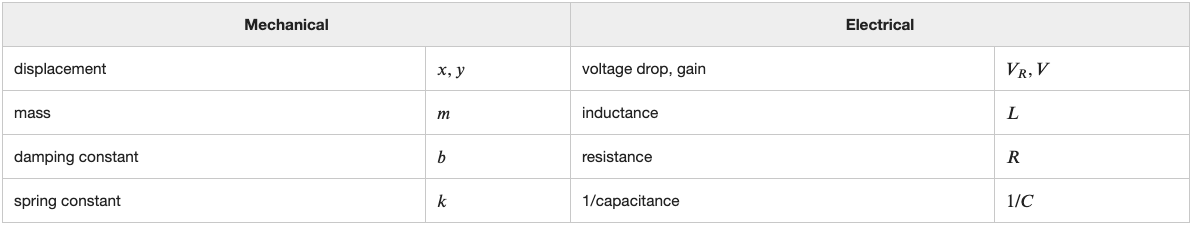
Fig.

Similarly, a harmonic oscillator (undamped) is analogous to a series LC circuit (no resistor).

We can also get the differential equations with \(V_L\) and \(V_C\) as inputs:

\[\begin{aligned} \displaystyle L{\color{blue}{\ddot{V}_ L}} +R{\color{blue}{\dot{V}_ L}}_+\frac{1}{C} {\color{blue}{V_ L}} &= \displaystyle L{\color{orange}{\ddot V}} \\ \displaystyle \displaystyle L{\color{blue}{\ddot{V}_ C}} +R{\color{blue}{\dot{V}_ C}} _+\frac{1}{C} {\color{blue}{V_ C}} &= \displaystyle \frac{1}{C} {\color{orange}{V}}. \end{aligned}\]

Recall the DE for the system response \(V_R\) and system input \(V\) is

\[\displaystyle P(D) V_ R\, =\, Q(D) V \quad \text{where} \\ \begin{aligned} P(D)\, &=\, L D^2 +R D+\frac{1}{C}\\ Q(D) &= RD. \end{aligned}\]

The complex gain for \(V_R\) is therefore

\[G_ R(\omega ) = \displaystyle \frac{Q(i\omega )}{P(i\omega )} = \displaystyle \frac{iR\omega }{\left(\frac{1}{C}-L\omega ^2\right)+iR\omega }.\]

Analogously, the complex gains for \(V_L\) and \(V_C\) are

\[\begin{aligned} G_L(\omega) &= \displaystyle \frac{-L\omega ^2 }{\left(\frac{1}{C}-L\omega ^2\right)+iR\omega } \\ G_C(\omega) &= \displaystyle \frac{\frac{1}{C} }{\left(\frac{1}{C}-L\omega ^2\right)+iR\omega }. \end{aligned}\]

Unit 5 Nonlinear DEs

12 Nonlinear DEs: Graphical methods

First order equations can be written in the standard form:

\[y' = f(x,y)\]

where \(f(x, y)\) is a function of the two variables \(x\) and \(y\).

For a differential equation \(y' = f(x, y)\), a slope field is a diagram which includes at each point \((x, y)\) a short line element whose slope is the value \(f(x, y)\).

Fig.

A solution curve is tangent to each line segment that it touches. The graph of a solution \(y_1(x)\) to the DE in the \(xy\)-plane is called a solution curve or an integral curve.

For a number \(C\), the \(C\)-isocline is the set of points in the \((x, y)\)-plane such that the solution curve through that point has slope \(C\).

The ODE says that the slope of the solution curve through a point \((x,y)\) is \(f(x,y)\), so the equation of the \(C\)-isocline is

\[f(x, y) = C.\]

The \(0\)-isocline is also called nullcline. The critical points of all solutions to the DE lie on the \(0\)-isocline.

Example. The organe curve shows the nullcline of \(y'=y^2-x\), which divides the plane into regions, and \(f(x, y)\) has constant sign on each region.

Fig.

Existence and uniqueness theorem for a first order (linear or nonlinear) ODE. Consider a first order ODE

\[y' = f(x,y).\]

For any point \((x_0, y_0)\) if \(f(x, y)\) and \(\frac{\partial f}{\partial y}\) are continuous near \((x_0, y_0)\), then there is unique solution to the first order DE through the point \((x_0, y_0)\). \(\square\)

As a consequence,

1. Solutions curves cannot cross.
2. Solutions curves cannot become tangent to one another (consider a neighborhood around (\(x_0, y_0\))).

13 Autonomous equations

An autonomous ODE is a differential equation that does not explicitly depend on the independent variable. The standard form for a first order autonomous equation is

\[\displaystyle \displaystyle \frac{dy}{dt} = f(y) \qquad (\text {instead of }\, f(t,y))\]

where the right hand side does not depend on \(t\).

Two consequences of the time invariance of an autonomous equation:

• Each isocline (in the \((t, y)\)-plane) consists of one or more horizontal lines.
• Solution curves are horizontal translations of one another.

Definition The values of \(y\) at which \(f(y) = 0\) are called critical points or equilibria of the autonomous equation \(\dot{y}=f(y)\).

If \(y_0\) is a critical point of an autonomous equation, then \(y=y_0\) is a constant solution. The \(0\)-isocline of an autonomous equation consists of all the constant solutions.

Recall that for any first order DE, the \(0\)-isocline divides the \((t, y)\)-plane into up regions, where \(f > 0\), and down regions, where \(f < 0\).

Fig.

To find the qualitative behaviour of solutions to \(\dot{y}=f(y)\), we follow two steps:

1. Find the critical points. That is, solve \(f(y) = 0\).
2. Determine the intervals of \(y\) in which \(f(y) > 0\) and in which \(f(y) < 0\). These are intervals in which solutions are increasing and decreasing respectively.

Definition. The phase line of a first order autonomous DE \(\dot{y} = f(y)\) is a plot of the \(y\)-axis with all critical points and with an arrow in each interval between the critical points indicating whether solutions increase or decrease.

Fig.

Logistic Equation. The simplest model for population \(y(t)\) is the ODE \(\dot{y} = ky\) for a positive growth constant \(k\), which is the birth rate minus the death rate of the population. This DE says that the rate of population growth is proportional to the current population, and we know the solution to be \(y(t) = Ce^{kt}\).

But realistically, if the population gets too large, then because of the competition for food and space, the population will grow less quickly. One simple way to model this is to adjust the growth rate from a constant function of \(y\) to a linearly decreasing function of \(y\). That is, let the growth rate be

\[\displaystyle \displaystyle k(y)=a-by\qquad (a,b>0 \, \text {constants}).\]

With the corrected growth rate, the DE becomes

\[\dot{y} = k(y) y = (a - by) y = ay -by^2 \qquad (a, b > 0).\]

This differential equation is called the logistic equation. It is nonlinear, autonomous equation.

A critical point \(x = a\) is called

• stable (blue color) if solutions starting near it move towards it,
• unstable (orange color) if solutions starting near it move away from it,
• semistable (black color) if the behavior depends on which side of the critical point starts.

Fig.

In the example of \(\dot{y} = 3y - y^2\), the critical points are 0 and 3. The phase line shows that \(0\) is unstable and \(3\) is stable.

Summary: steps for understanding solutions to \(\dot{y} = f(y)\) qualitatively.

1. Find the critical points by solving \(f(y)=0\).
2. Determine the intervals of \(y\) in which \(f(y) > 0\) and \(f(y) < 0\).
3. Draw the phase line, which consists of a line marked with \(-\infty\), the critical points, \(+\infty\), and arrows between these.
4. Solutions starting at a critical point are constant.
5. Other solutions tend to the limit that the arrow points to as \(t\) increases, and tend to the limit that the arrow originates from as \(t\) decreases.

Now consider if this population is also harvested at a constant rate \(h\), we add a term to the logistic equation to include the effect of harvesting:

\[\dot{y}=ay-by^2-h \qquad (a,b>0,\, h\geq 0)\qquad (\text {with harvesting})\]

The quadratic function \(ay-by^2-h\) gets decreased by \(h\) compared with \(ay-by^2\), it will have only one critical point when it is tangent to \(y\)-axis as shown in the figure below.

Fig.

Let us draw the picture of the critical points change over \(h\) for the DE \(\displaystyle 3y-y^2-h\qquad (h\geq 0).\)

Fig.

If we draw phase lines at all \(h\)-values, we get a diagram which is called a bifurcation diagram,

Fig.

Definition. A bifurcation diagram of a family of autonomous equations depending on a parameter \(h\) is a plot of the values of the critical points as functions of $h$, along with one arrow in each region in the \((h,y)\)-plane defined by the curve, indicating whether solutions are increasing or decreasing in that regions.

14 Numerical Methods

Euler’s Method.

Given an initial value problem

\[y'\, =\, f(t,y)\qquad y(t_0)=y_0,\]

and a choice of step size \(h\), the Euler’s method gives an approximation to the solution curve between \(t=t_0\) and \(t = t_0 + (n+1)h\), by a sequence of line segments connecting the points \(\, (t_0,y_0),\, (t_1,y_1),\, \ldots \, (t_ n,y_ n), \, (t_{n+1},y_{n+1}),\,\) where for each \(0 \leq k \leq n\),

\[\begin{aligned} t_{k+1} &= t_k + h \\ y_{k+1} &= y_ k+h f(t_ k,y_ k). \end{aligned}\]

Fig.

Runge-Kutta methods.

Integration	Differential equation	Error
left Riemann sum	Euler’s method	\(O(h)\)
trapezoid rule	second-order Runge-Kutta method (RK2)	\(O(h^2)\)
Simpson’s rule	fourth-order Runge-Kutta method (RK4)	\(O(h^4)\)

RK2. It is also called the midpoint method or the modified Euler method.

Fig.

1. Starting from \((t_0, y_0)\), look ahead to see where one step of Euler’s method would land, call it \((t_1, \tilde{y}_1)\).

2. Find the midpoint between the starting point and the temporary point: \(\, \left( \frac{t_0+t_1}{2}, \frac{y_0+\tilde{y}_1}{2} \right).\)

3. Use the slope at this midpoint to find \(y_1\)

   \[y_1\, =\, y_0 +h f\left( \frac{t_0+t_1}{2}, \frac{y_0+\tilde{y}_1}{2} \right).\]

Repeat the steps above using \((t_1, y_1)\) as the starting point.

Here is the summary of the equations:

\[\begin{aligned} t_1 &= t_0 + h \\ \tilde{y}_1 &= y_0 + h f(t_0, y_0) \\ y_1 &= y_0+ h f\left(\frac{t_0+t_1}{2},\frac{y_0+\tilde{y}_1}{2}\right) \\ (t_0, y_0) &\mapsto \displaystyle \left(t_1, y_1\right). \end{aligned}\]

---