Introductory Lectures on Convex Optimization 2
Chapter 2 of Introductory Lectures on Convex Optimization.
2 Smooth convex optimization
We have seen that, in general, the gradient method converges only to a stationary point of function \(f\), which motivates us to find a class of function \(\mathcal{F}\) such that
Assumption 2.1.1 For any \(f \in \mathcal{F}\) the first-order optimality condition, \(f'(x)=0\), is sufficient for a point to be a global solution.
We introduce another invariant operation for the hypothetical class \(\mathcal{F}\).
Assumption 2.1.2 If \(f_1, f_2 \in \mathcal{F}\) and \(\alpha, \beta \geq 0\), then \(\alpha f_1 + \beta f_2 \in \mathcal{F}\).
Let’s introduce one basic element
Assumption 2.1.3 Any linear function \(f(x) = \alpha + \langle a , x \rangle\) belongs to \(\mathcal{F}\).
The reason is obvious, because for a linear function, \(f'(x) = 0\) implies that it must be a constant function, thus any point in its domain is the optimal solution.
Now let’s see what kind of conclusions we can make about our hypothetical class \(\mathcal{F}\). Consider \(f \in \mathcal{F}\) and for a fixed point \(x_0 \in \mathbb{R}^n\) the function
\[\phi ( y ) = f ( y ) - \left\langle f ^ { \prime } \left( x _ { 0} \right) ,y \right\rangle\]is a non-negative linear combination of \(f(y)\) and linear function \(-\langle f ^ { \prime } \left( x _ { 0} \right) ,y \rangle\) thus \(\phi \in \mathcal{F}\). Note that
\[\phi ^ { \prime } ( y ) \vert _ { y = x _ { 0} } = f ^ { \prime } \left( x _ { 0} \right) - f ^ { \prime } \left( x _ { 0} \right) = 0\]Hence, in view of assumtion 2.1.1 we have for any \(y \in \mathbb{R}^n\) we have \(\phi ( y ) \geq \phi \left( x _ { 0} \right) = f \left( x _ { 0} \right) - \left\langle f ^ { \prime } \left( x _ { 0} \right) ,x _ { 0} \right\rangle\)
Hence we conclude that
\[f ( y ) \geq f \left( x _ { 0} \right) + \left\langle f ^ { \prime } \left( x _ { 0} \right) ,y - x _ { 0} \right\rangle\]This inequality defines the class of differentiable convex functions.
Defintion 2.1.1 A continuously differentiable function \(f(x)\) is called convex on \(\mathbb{R}^n\) (\(f \in \mathcal { F } ^ { 1} \left( \mathbb{R} ^ { n } \right)\)) if for any \(x, y \in \mathbb{R}^n\) we have
\[f ( y ) \geq f ( x ) + \left\langle f ^ { \prime } ( x ) ,y - x \right\rangle\]Theorem 2.1.1 If \(f \in \mathcal { F } ^ { 1} \left( \mathbb{R} ^ { n } \right)\) and \(f'(x^*) = 0\) then \(x^*\) is the global minimum of \(f(x)\) on \(\mathbb{R}^n\).
Lemma 2.1.1 If \(f_1, f_2 \in \mathcal { F } ^ { 1} \left( \mathbb{R} ^ { n } \right)\) and \(\alpha, \beta \geq 0\) then function \(f = \alpha f_1 + \beta f_2\) also belongs to \(\mathcal { F } ^ { 1} \left( \mathbb{R} ^ { n } \right)\).
Lemma 2.1.2 If \(f \in \mathcal { F } ^ { 1} \left( \mathbb{R} ^ { m } \right), b \in \mathbb{R} ^ { m }\) and \(A : \mathbb{R}^n \rightarrow \mathbb{R}^m\) then
\[\phi ( x ) = f ( A x + b ) \in \mathcal { F } ^ { 1} \left( R ^ { n } \right)\]Proof: Let \(x, y \in \mathbb{R}^n\) and denote \(\bar{x} = Ax + b, \bar{y} = Ay + b\). We have \(f ( \overline { y } ) \geq f ( \overline { x } ) + \left\langle f ^ { \prime } ( \overline { x } ) ,\overline { y } - \overline { x } \right\rangle\). Also note that \(\phi(y) = f(\bar{y}), \phi(x) = f(\bar{x})\), what remains is to show that \(\phi(y) \geq \phi(x) + \langle \phi(x)', y-x \rangle\).
:black_medium_square:
We provide several equivalent definitions of convex function.
Theorem 2.1.2 Continously differentiable function \(f\) belongs to the class \(\mathcal { F } ^ { 1} \left( \mathbb{R} ^ { n } \right)\) if and only if for any \(x, y \in \mathbb{R}^n\) and \(\alpha \in [0, 1]\) we have
\[f ( \alpha x + ( 1- \alpha ) y ) \leq \alpha f ( x ) + ( 1- \alpha ) f ( y ).\]Proof: Denote \(x _ { \alpha } = \alpha x + ( 1- \alpha ) y\) and let \(f \in \mathcal { F } ^ { 1} \left( \mathbb{R} ^ { n } \right)\). Then
\[\left.\begin{array} { l l } { f \left( x _ { \alpha } \right) } & { \leq f ( y ) + \left\langle f ^ { \prime } \left( x _ { \alpha } \right) ,y - x _ { \alpha } \right\rangle } & { = f ( y ) + \alpha \left\langle f ^ { \prime } \left( x _ { \alpha } \right) ,y - x \right\rangle } \\ { f \left( x _ { \alpha } \right) } & { \leq f ( x ) + \left\langle f ^ { \prime } \left( x _ { \alpha } \right) ,x - x _ { \alpha } \right\rangle } & { = f ( x ) - ( 1- \alpha ) \left\langle f ^ { \prime } \left( x _ { \alpha } \right) ,y - x \right\rangle } \end{array} \right.\]Multiplying first inequality by \(1 - \alpha\) and the second one by \(\alpha\) and adding the results, we get \(f ( \alpha x + ( 1- \alpha ) y ) \leq \alpha f ( x ) + ( 1- \alpha ) f ( y ).\)
Let \(f ( \alpha x + ( 1- \alpha ) y ) \leq \alpha f ( x ) + ( 1- \alpha ) f ( y )\) be true for all \(x, y \in \mathbb{R}^n\) and \(\alpha \in [0, 1)\). Then
\[\left.\begin{aligned} f ( y ) & \geq \frac { 1} { 1- \alpha } \left[ f \left( x _ { \alpha } \right) - \alpha f ( x ) \right] = f ( x ) + \frac { 1} { 1- \alpha } \left[ f \left( x _ { \alpha } \right) - f ( x ) \right] \\ & = f ( x ) + \frac { 1} { 1- \alpha } [ f ( x + ( 1- \alpha ) ( y - x ) ) - f ( x ) ] \end{aligned} \right.\]using first order Taylor expansion and tending \(\alpha\) to 1, we get \(f ( y ) \geq f ( x ) + \left\langle f ^ { \prime } ( x ) ,y - x \right\rangle\).
It is worthwhile mentioning that even without the differentiability assumption, the definition still holds.
Theorem 2.1.3 Continuously differentiable function \(f\) belongs to the class \(\mathcal { F } ^ { 1} \left( \mathbb{R} ^ { n } \right)\) if and only if we have
\[\left\langle f ^ { \prime } ( x ) - f ^ { \prime } ( y ) ,x - y \right\rangle \geq 0\]Proof: \(\mathcal { F } ^ { 1} \left( \mathbb{R} ^ { n } \right) \rightarrow\) \(\left\langle f ^ { \prime } ( x ) - f ^ { \prime } ( y ) ,x - y \right\rangle \geq 0\) is straightforward.
Let \(\left\langle f ^ { \prime } ( x ) - f ^ { \prime } ( y ) ,x - y \right\rangle \geq 0\) hold for all \(x, y \in \mathbb{R}^n\) and denote \(x _ { \tau } = x + \tau ( y - x )\). Then
\[\left.\begin{aligned} f ( y ) & = f ( x ) + \int _ { 0} ^ { 1} \left\langle f ^ { \prime } ( x + \tau ( y - x ) ) ,y - x \right) d \tau \\ & = f ( x ) + \left\langle f ^ { \prime } ( x ) ,y - x \right\rangle + \int _ { 0} ^ { 1} \left\langle f ^ { \prime } \left( x _ { \tau } \right) - f ^ { \prime } ( x ) ,y - x \right\rangle d \tau \\ & = f ( x ) + \left\langle f ^ { \prime } ( x ) ,y - x \right\rangle + \int _ { 0} ^ { 1} \frac { 1} { \tau } \left\langle f ^ { \prime } \left( x _ { \tau } \right) - f ^ { \prime } ( x ) ,x _ { \tau } - x \right) d \tau \\ & \geq f ( x ) + \left\langle f ^ { \prime } ( x ) ,y - x \right\rangle \end{aligned} \right.\]Now we consider the twice differentiable function class \(\mathcal { F } ^ {2} \left( \mathbb{R} ^ { n } \right)\).
Theorem 2.1.4 Twice continuously differentiable function \(f\) belongs to \(\mathcal { F } ^ { 2} \left( \mathbb{R} ^ { n } \right)\) if and only if for any \(x \in \mathbb{R}^n\) we have
\[f''(x) \succeq 0\]Proof: Let \(f \in \mathcal { F } ^ { 2} \left( \mathbb{R} ^ { n } \right)\) and \(x_\tau = x + \tau s\), \(\tau > 0\). Then in the view of Theorem 2.1.3, we have
\[\left.\begin{aligned} 0& \leq \frac { 1} { \tau } \left\langle f ^ { \prime } \left( x _ { \tau } \right) - f ^ { \prime } ( x ) ,x _ { \tau } - x \right\rangle = \left\langle f ^ { \prime } \left( x _ { \tau } \right) - f ^ { \prime } ( x ) ,s \right\rangle \\ & = \left\langle \int_0 ^\tau d f^{\prime}(x + \lambda s), s \right\rangle \\ &= \int_0 ^\tau \langle f ^ { \prime \prime } ( x + \lambda s ) d(x + \lambda s), s \rangle\\ &= \int_0^\tau \left\langle f ^ { \prime \prime } ( x + \lambda s ) s ,s \right\rangle d \lambda \end{aligned} \right.\]and tending \(\tau\) to 0 we get \(f''(x) \succeq 0\).
Let \(f''(x) \succeq 0\) hold and \(s = y-x\). Then
\[\left.\begin{aligned} f ( y ) & = f ( x ) + \int _ { 0} ^ { 1} \left\langle f ^ { \prime } ( x + \tau ( y - x ) ) ,y - x \right) d \tau \\ & = f ( x ) + \left\langle f ^ { \prime } ( x ) ,y - x \right\rangle + \int _ { 0} ^ { 1} \left\langle f ^ { \prime } \left( x _ { \tau } \right) - f ^ { \prime } ( x ) ,y - x \right\rangle d \tau \\ &= f ( x ) + \left\langle f ^ { \prime } ( x ) ,y - x \right\rangle + \int _ { 0} ^ { 1} \int_0^\tau \left\langle f ^ { \prime \prime } ( x + \lambda s ) s ,s \right\rangle d \lambda d \tau \\ & \geq f(x) + \langle f'(x), y-x \rangle. \end{aligned} \right.\]:black_medium_square:
Examples of differentiable convex function.
According to Lemma 2.1.2, \(f ( x ) = \sum _ { i = 1 } ^ { m } e ^ { \alpha _ { i } + \left\langle a _ { i } , x \right\rangle }\) and \(f ( x ) = \sum _ { i = 1 } ^ { m } \left\vert \left\langle a _ { i } , x \right\rangle - b _ { i } \right\vert ^ { p }\) are all convex functions.
The differentiability iteself cannot ensure any special topological properties of convex functions. Therefore we need to consider the problem classes with Lipschitz continuous derivatives of a certain order.
Theorem 2.1.5 All conditions below, holding for all \(x, y \in \mathbb{R}^n\) and \(\alpha \in [0, 1]\), are equivalent to inclusion \(f \in \mathcal { F } _ { L } ^ { 1,1 } \left( \mathbb{R} ^ { n } \right)\):
\[\text{(1)}\quad 0 \leq f ( y ) - f ( x ) - \left\langle f ^ { \prime } ( x ) , y - x \right\rangle \leq \frac { L } { 2 } \| x - y \| ^ { 2 }\] \[\text{(2)}\quad f ( x ) + \left\langle f ^ { \prime } ( x ) , y - x \right\rangle + \frac { 1 } { 2 L } \left\| f ^ { \prime } ( x ) - f ^ { \prime } ( y ) \right\| ^ { 2 } \leq f ( y )\] \[\text{(3)}\quad \frac { 1 } { L } \left\| f ^ { \prime } ( x ) - f ^ { \prime } ( y ) \right\| ^ { 2 } \leq \left\langle f ^ { \prime } ( x ) - f ^ { \prime } ( y ) , x - y \right\rangle\] \[\text{(4)}\quad \left\langle f ^ { \prime } ( x ) - f ^ { \prime } ( y ) , x - y \right\rangle \leq L \| x - y \| ^ { 2 }\] \[\begin{aligned} \alpha f ( x ) + ( 1 - \alpha ) f ( y ) \geq & f ( \alpha x + ( 1 - \alpha ) y ) \\ & + \frac { \alpha ( 1 - \alpha ) } { 2 L } \left\| f ^ { \prime } ( x ) - f ^ { \prime } ( y ) \right\| ^ { 2 } \end{aligned}\] \[\begin{aligned} \alpha f ( x ) + ( 1 - \alpha ) f ( y ) \leq & f ( \alpha x + ( 1 - \alpha ) y ) \\ & + \alpha ( 1 - \alpha ) \frac { L } { 2 } \| x - y \| ^ { 2 } \end{aligned}\]Proof: (1) follows from the definition of convex functions and Lemma 1.2.3. To prove (2), let us fix \(x\) and consider the function
\[\phi ( y ) = f ( y ) - \left\langle f ^ { \prime } \left( x \right) , y \right\rangle\]Note that \(\phi \in \mathcal { F } _ { L } ^ { 1,1 } \left( R ^ { n } \right)\) and its optimal point is \(y^* = x\) and in the view of (1), we have
\[\begin{aligned} \phi \left( x \right) = \min_{v} \phi(v) \leq \min_{v} \left[ \phi(y) + \langle \phi^{\prime}(y), v - y\rangle + \frac{1}{2} L \| v - y \|^2\right] \end{aligned}\]where the right most function get its minimum at \(v = y - \frac { 1 } { L } \phi ^ { \prime } ( y )\) and replacing \(v\) we get (2).
We get (3) from (2) by adding two copies of it with \(x\) and \(y\) interchanged.
Applying to (3) Cauchy-Schwartz inequality we get \(\left\| f ^ { \prime } ( x ) - f ^ { \prime } ( y ) \right\| \leq L \| x - y \|\), the definition of one order Lipschitz continuous gradient, i.e., (1).
We can get (4) from (1) by adding two copies of it with \(x\) and \(y\) interchanged.
To get (1) from (4) we apply integration:
\[\begin{aligned} f ( y ) - f ( x ) - \left\langle f ^ { \prime } ( x ) , y - x \right\rangle & = \int _ { 0 } ^ { 1 } \left\langle f ^ { \prime } ( x + \tau ( y - x ) ) - f ^ { \prime } ( x ) , y - x \right\rangle d \tau \\ & \leq \frac { 1 } { 2 } L \| y - x \| ^ { 2 } \end{aligned}\]Theorem 2.1.6 Two times continuously differentiable function \(f\) belongs to \(\mathcal { F } _ { L } ^ { 2,1 } \left( R ^ { n } \right)\) if and only if for any \(x \in R ^ { n }\) we have
\[0 \preceq f ^ { \prime \prime } ( x ) \preceq L I _ { n }.\]Proof: According to (4) in Theorem 2.1.5,
\[\left.\begin{aligned} \tau L \|s\|^2 &\geq \frac { 1} { \tau } \left\langle f ^ { \prime } \left( x + \tau s \right) - f ^ { \prime } ( x ) ,x + \tau s - x \right\rangle \\ &= \left\langle f ^ { \prime } \left( x _ { \tau } \right) - f ^ { \prime } ( x ) ,s \right\rangle \\ & = \left\langle \int_0 ^\tau d f^{\prime}(x + \lambda s), s \right\rangle \\ &= \int_0 ^\tau \langle f ^ { \prime \prime } ( x + \lambda s ) d(x + \lambda s), s \rangle\\ &= \int_0^\tau \left\langle f ^ { \prime \prime } ( x + \lambda s ) s ,s \right\rangle d \lambda \end{aligned} \right.\]hence we have
\[L \|s\|^2 \geq \frac{1}{\tau} \int_0^\tau \left\langle f ^ { \prime \prime } ( x + \lambda s ) s ,s \right\rangle d \lambda\]i.e.
\[f ^ { \prime \prime } ( x ) \preceq L I _ { n }\]If we have
\[f ^ { \prime \prime } ( x ) \preceq L I _ { n }\]then
\[\left.\begin{aligned} L \|y - x\|^2 &\geq \int_0^1 \left\langle f ^ { \prime \prime } ( x + \lambda (y-x) ) (y-x) , y-x \right\rangle d \lambda \\ &= \left\langle f ^ { \prime } \left(y \right) - f ^ { \prime } ( x ) , y-x \right\rangle. \end{aligned}\right.\]Remark: This theorem states
\[f ^ { \prime \prime } ( x ) \preceq L I _ { n } \Leftrightarrow \left\langle f ^ { \prime } \left(y \right) - f ^ { \prime } ( x ) , y-x \right\rangle \leq L \|y - x\|^2\]Similarly, we could prove
\[f ^ { \prime \prime } ( x ) \succeq \mu I _ { n } \Leftrightarrow \left\langle f ^ { \prime } \left(y \right) - f ^ { \prime } ( x ) , y-x \right\rangle \geq \mu \|y - x\|^2.\]2.1.2 Lower complexity bounds for \(\mathcal { F } _ { \boldsymbol { L } } ^ { \infty , \mathbf { 1 } } \left( \boldsymbol { R } ^ { n } \right)\)
Assumption 2.1.4 An iterative method \(\mathscr{M}\) generates a sequence of test points \(\{ x_k \}\) such that
\[x_{k} \in x_{0}+\operatorname{Lin}\left\{\nabla f\left(x_{0}\right), \ldots, \nabla f\left(x_{k-1}\right)\right\}, \quad k \geq 1\]Consider the following family of quadratic functions with a fixed constant \(L > 0\)
\[f_k (x) = \frac{L}{4}\left[ \langle x, A_k x \rangle - \langle x, e_1 \rangle \right]\]where
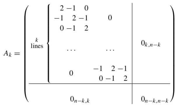
Fig. \(A_k\)
\(A_k\) is a tri-diagonal matrix. Thus \(0 \preceq \nabla^{2} f_{k}(x) \preceq L I_{n}\) and \(f_{k}(\cdot) \in \mathscr{F}_{L}^{\infty, 1}\left(\mathbb{R}^{n}\right), 1 \leq k \leq n\). Therefore, the equation
\[\nabla f_{k}(x)= 2A_{k} x-e_{1}=0\]has unique solution:
\[\bar{x}_{k}^{(i)}=\left\{\begin{array}{cc}{1-\frac{i}{k+1},} & {i=1 \ldots k} \\ {0,} & {k+1 \leq i \leq n}\end{array}\right.\]Hence, the optimal value of the function \(f_k\) is
\[\begin{align} f_k^* &= \frac{L}{4}\left[ \langle \bar{x}, A_k \bar{x} \rangle - \langle \bar{x}, e_1 \rangle \right] \\ &= \frac{L}{4}\left[ \langle \bar{x}, \frac{1}{2} e_1 \rangle - \langle \bar{x}, e_1 \rangle \right] \\ &= \frac{L}{8}\left(-1+\frac{1}{k+1}\right) \end{align}\]Note that
\[\sum_{i=1}^{k} i^{2}=\frac{k(k+1)(2 k+1)}{6} \leq \frac{(k+1)^{3}}{3}\]Therefore,
\[\begin{aligned}\left\|\bar{x}_{k}\right\|^{2} &=\sum_{i=1}^{n}\left(\bar{x}_{k}^{(i)}\right)^{2}=\sum_{i=1}^{k}\left(1-\frac{i}{k+1}\right)^{2} \\ &=k-\frac{2}{k+1} \sum_{i=1}^{k} i+\frac{1}{(k+1)^{2}} \sum_{i=1}^{k} i^{2} \\ & \leq k-\frac{2}{k+1} \cdot \frac{k(k+1)}{2}+\frac{1}{(k+1)^{2}} \cdot \frac{(k+1)^{3}}{3}=\frac{1}{3}(k+1) \end{aligned}\]Let \(\mathbb{R}^{k, n}=\left\{x \in \mathbb{R}^{n} \vert x^{(i)}=0, k+1 \leq i \leq n\right\}\). Then for any \(x \in \mathbb{R}^{k, n}\) we have
\[f_{p}(x) = f_{k}(x), \quad p=k, \ldots, n\]since \(\langle x, A_p x \rangle \in \mathbb{R}^{k, n}\) for all \(x \in \mathbb{R}^{k, n}\).
Now let us fix \(p, k \leq p \leq n\).
Lemma 2.1.5 Let \(x_0 = 0\). Then for any sequence \(\left\{x_{k}\right\}_{k=0}^{p}\) satisfying the condition
\[x_{k} \in \mathscr{L}_{k} \stackrel{\mathrm{def}}{=} \operatorname{Lin}\left\{\nabla f_{p}\left(x_{0}\right), \ldots, \nabla f_{p}\left(x_{k-1}\right)\right\}\]we have \(\mathscr{L}_{k} \subseteq \mathbb{R}^{k, n}\).
Proof Since \(x_0 = 0\), we have \(\nabla f_{p}\left(x_{0}\right)=-\frac{L}{4} e_{1} \in \mathbb{R}^{1, n}\). Thus \(\mathscr{L}_1 = \mathbb{R}^{1,n}\). Let \(\mathscr{L}_{k} \subseteq \mathbb{R}^{k, n}\) for some \(k < p\). Since \(A_p\) is tri-diagonal for any \(x \in \mathbb{R}^{k,n}\) we have \(\nabla f_{p}(x) \in \mathbb{R}^{k+1, n}\). Therefore \(\mathscr{L}_{k+1} \subseteq \mathbb{R}^{k+1, n}\). \(\square\)
Remark: \(A_p x \in \mathbb{R}^{k+1, n}\) for \(x \in \mathbb{R}^{k, n}\) and \(p \geq k\), just consider the element in \(k+1\)-row and \(k\)-column of \(A_p\).
Corollary 2.1.1 For any sequence \(\{x_k\}_{k=0}^p\) with \(x_0 = 0\) and \(x_k \in \mathscr{L}_{k}\), we have
\[f_{p}\left(x_{k}\right) \geq f_{k}^{*}.\]Proof: Since \(x_k \in \mathscr{L}_{k} \subseteq \mathbb{R}^{k, n}\) and therefore \(f_{p}\left(x_{k}\right)=f_{k}\left(x_{k}\right) \geq f_{k}^{*}\).
Theorem 2.1.7 For any \(k, 1 \leq k \leq \frac{1}{2}(n-1)\), and any \(x_{0} \in \mathbb{R}^{n}\) there exists a function \(f \in \mathscr{F}_{L}^{\infty, 1}\left(\mathbb{R}^{n}\right)\) such that for any first-order method \(\mathscr{M}\) satisfying Assumption 2.1.4 we have
\[\begin{array}{l}{f\left(x_{k}\right)-f^{*} \geq \frac{3 L\left\|x_{0}-x^{*}\right\|^{2}}{32(k+1)^{2}}}, \\ {\left\|x_{k}-x^{*}\right\|^{2} \geq \frac{1}{8}\left\|x_{0}-x^{*}\right\|^{2}},\end{array}\]where \(x^*\) is the minimum of the function \(f\) and \(f^* = f(x^*)\).